Lecture 7: Introduction to R for Hypothesis Testing
Damien Dupré | DCU Business School
Previously in STA1005
Brief Introduction
Modern data science uses free and open-source languages:
Proprietary languages (e.g., Matlab, Stata, SAS) and software (e.g., SPSS) are outdated
Main open-source computer languages for data science are Python and R
While Python is the most used language by computer engineers for web and app development, R has some advantages:
Easy to write, to read and to use
Focused on reports and journal papers with reproducibility
Advanced statistical packages
Friendly and open community
So let’s useR!
1. R and RStudio
What are R and RStudio?
There are some key concepts you need to understand and to remember:
R is the name of the language
RStudio is the name of the upgraded interface to write R code
R is usually used via RStudio and first time users often confuse the two. At its simplest, R is like a car’s engine while RStudio is like a car’s dashboard.
Most of the R code displayed in this lecture is included in these slides. Rather than typing it manually, open these slides in another tab to copy-paste the code.
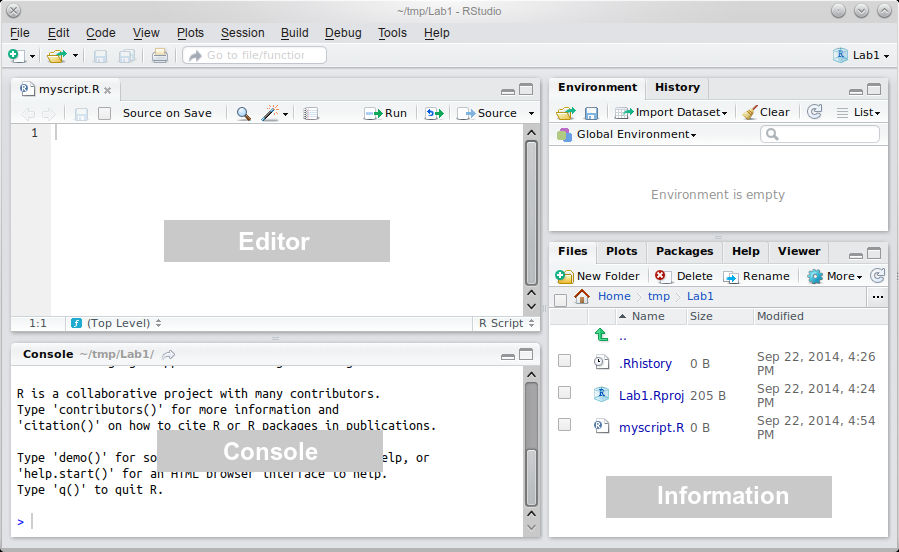
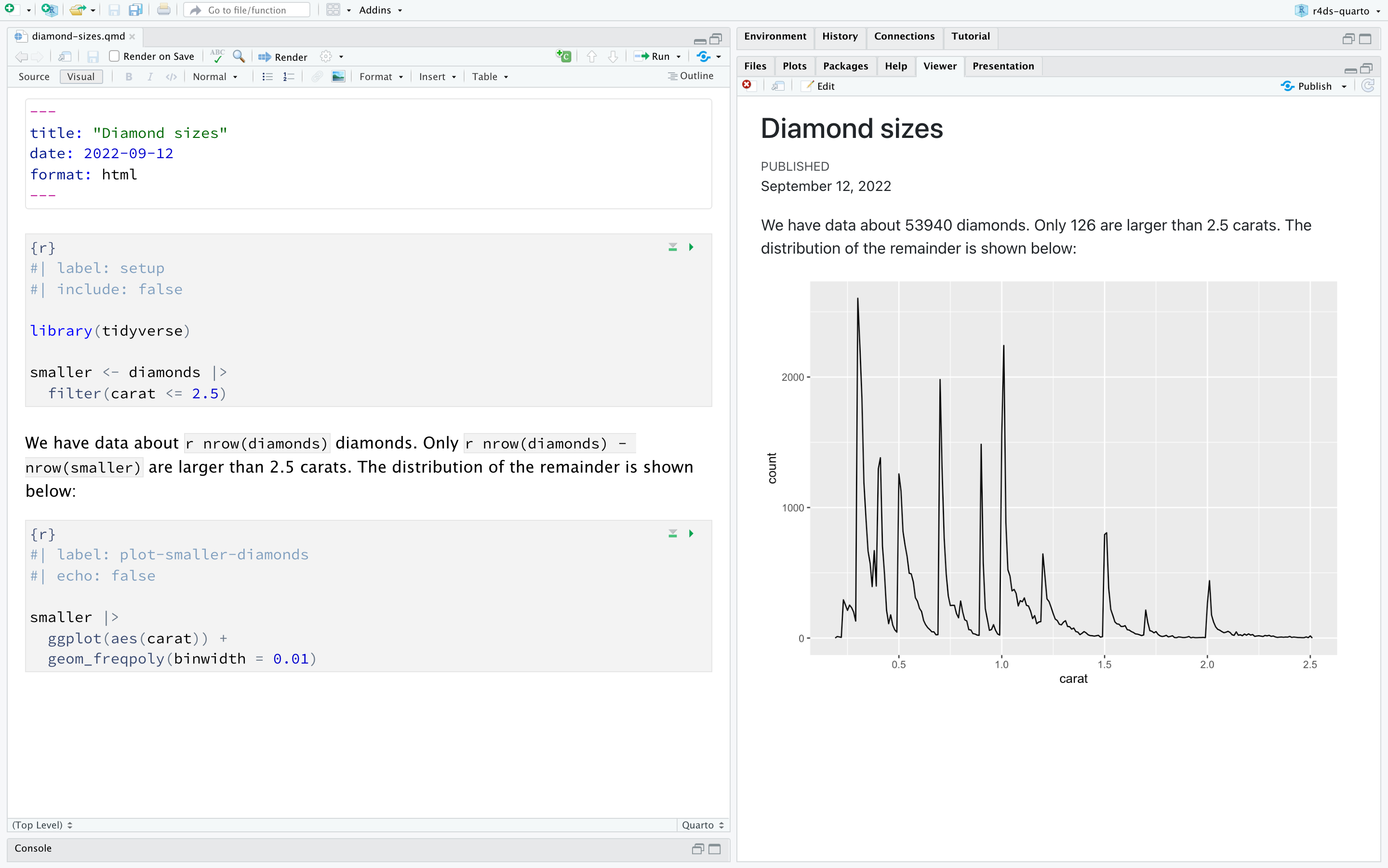
When you create a new project, you will see the following 3 windows (also called panes):
Console: where the results are printed
Workspace: where the objects are stored
Files, Plots, Package, Help and Viewer: where data science materials are
The last window Code Editor opens when creating a new R Script
Console: R’s Heart
The console displays
What has been run,
The results (or some parts) of what has been run, and
The status of the R process.
Console: R’s Heart
The Status of R is indicated by the symbol in the console prompt:
> means ready to process code
+ means incomplete command (escape with Esc)
🛑 at the top right corner means the console is busy processing your code
The Console Doesn’t Save!
You can execute code by typing it directly into the Console. However, it will not be saved. And if you make a mistake you will have to re-type everything all over again.
Instead, write all your code in a document (R script or Quarto file) in the Code Editor.
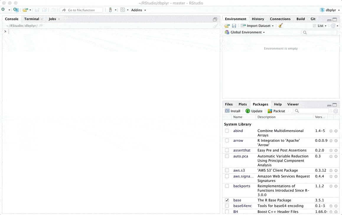
Environment: R’s Brain
The Environment tab of this pane shows you the names of all the data objects (like vectors, matrices, and data frames) that you have defined in your current R session.
You can also see information like the number of observations and rows in data objects.
Files / Plots / Packages / Help
The Files panel gives access to the file directory.
The Plots panel shows all your plots. There are buttons for opening the plot in a pop up and exporting as a pdf or jpeg.
The Packages shows a list of all the R packages installed on the local or remote machine and indicates whether or not they are currently loaded.
With the Help menu for R functions you can access essential information to use them. Just have a look at some of them by pressing F1 with the cursor on the function, using the help() function, or by typing ? followed by the function name such as:
help(seq)?seq
Code Editor: R’s Nervous System
It makes the link between all the previous panes and allows you to reproduce actions and behaviours.
You can open as many R Script / Quarto files as you want.
These documents are the only documents that have to be saved. No need to save your data, figures and calculations as you can reproduce them every time instantaneously with the code.
Code Editor: R’s Nervous System
Save your eyes and look like a nerd by changing the code’s appearance
3. The Basics of R Code
What are .R and .qmd files?
.R is the extension for an R script (document including R code):
Click File > New File > R Script in RStudio
Includes code which can be active or inactive (after #)
Used for code testing
Example of non-active code
# non active code
Example of active code
paste("active", "code")
[1] "active code"
1+1# everything after `#` is non active and is used for comments
[1] 2
What are .R and .qmd files?
.qmd is the extension for a Quarto file:
Click File > New File > Quarto document… in RStudio
Refers to a document that includes code and text
Generates a specific type of output
.html (web page, slides, books, and dashboards)
.pdf (Academic LaTex papers and reports)
.doc (MS Word documents)
How to Run R Code?
In an R Script, place your cursor anywhere on the line you want to run and either:
Press Ctrl & Enter (Win)
Press command & Enter (Mac)
Click the Run button on RStudio’s interface
What are R packages?
R packages extend the functionality of R. They are written by a worldwide community of R users and can be downloaded for free from the internet.
A good analogy for R packages are like apps you can download onto a mobile phone.
What are R packages?
R: A new phone
R Packages: Apps you can download
What are R packages?
Say you have purchased a new phone, to use Instagram you need to install the app once and to open the app every time to use it.
The process is very similar for using an R package. You need to:
Install the package with the function install.packages().
install.packages("praise")
“Load” the package with the function library().
library(praise)
Once the package is loaded you can use all the functions from this package such as:
praise()
Live Demo
️ Your Turn!
Open an R Script in RStudio. In this document:
Use line 1 to install the package “praise”
install.packages("praise")
Use line 2 to load the library praise
library(praise)
Use line 3 to run the function praise() as it is, without arguments
praise()
05:00
Calling Functions
Functions are algorithms (or lines of code) which transform data to something else. For example, the function lm(), uses data to compute the result of a linear regression model.
Functions have a name and several arguments that require some information.
For example, the function seq() makes a sequence of numbers:
The first argument from is the number starting the sequence
The second argument to is the last number of the sequence
seq(from =1, to =10)
[1] 1 2 3 4 5 6 7 8 9 10
Warning
Arguments don’t need to be explicitly called, they can also be matched by position:
seq(1, 10)
[1] 1 2 3 4 5 6 7 8 9 10
Assign Values to Objects in R
Usually the arguments of functions expect an Object name to access the data.
An object is a box that can include anything (e.g., values, dataframes, figures, models, functions, …) and has a name that you have to choose.
Assign Values to Objects in R
To create an object, you need to assign something to a name using the <- operator. If you type the name of the object, R will print out its content.
x <-4x
[1] 4
seq(x, 10)
[1] 4 5 6 7 8 9 10
Assign Values to Objects in R
It is very important to distinguish values and objects in R:
Type
Class
Example
Number
Numeric Value
1, 2, ...
Word with quotes
Character Value
"one", "two", ...
Word without quotes
Object Name
function name, data name, ...
Assign Values to Objects in R
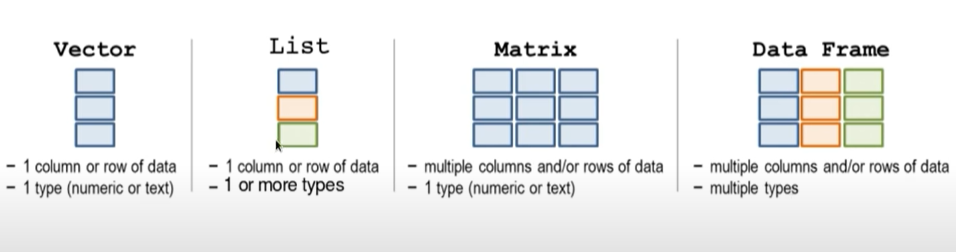
These types of values are then stored in different objects:
Different R Objects
All object assignments have the same form:
object_name <- object_content
You want your object names to be descriptive, so you will need a convention for multiple words. I recommend snake_case where you separate lower-case words with _.
Once it works, try changing the values in my_power and my_knowledge to customise the chart.
05:00
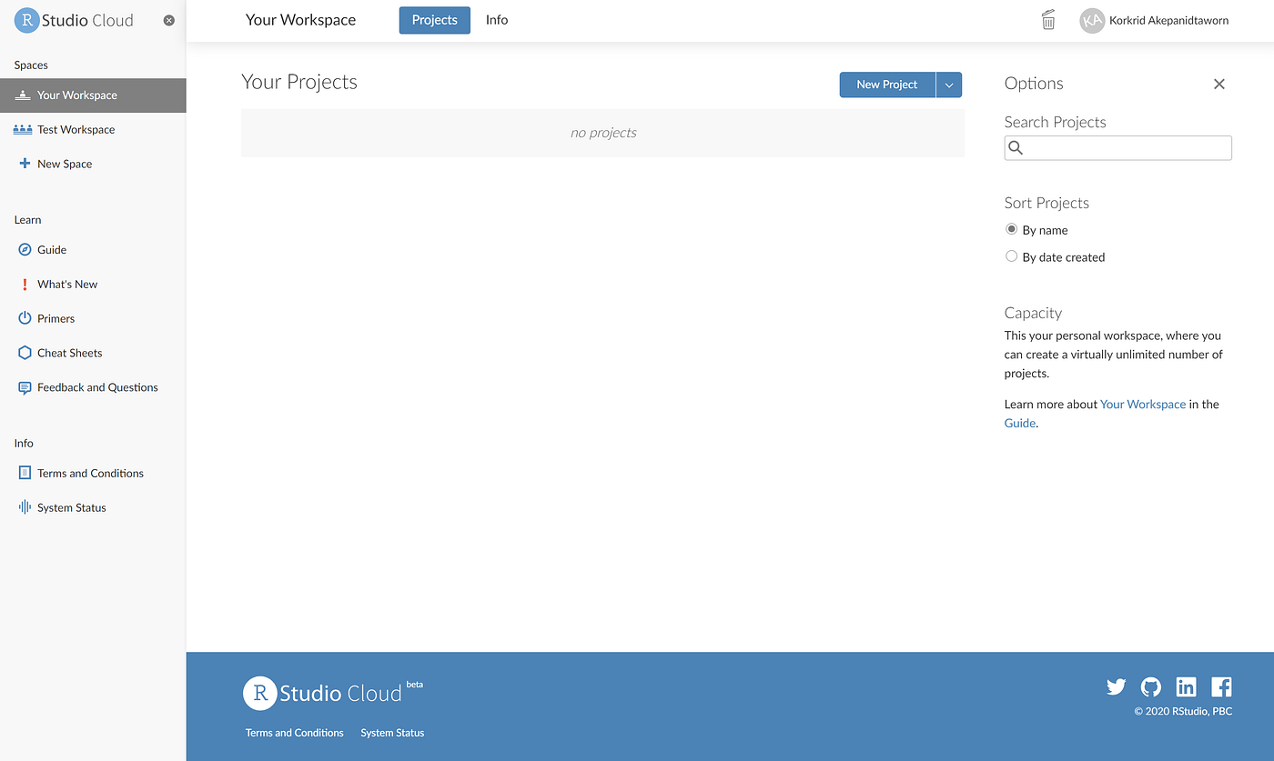
4. Access Data in Posit Cloud
Open your Data as R Object (1)
Posit Cloud is a free remote computer, the computing is not run on your computer.
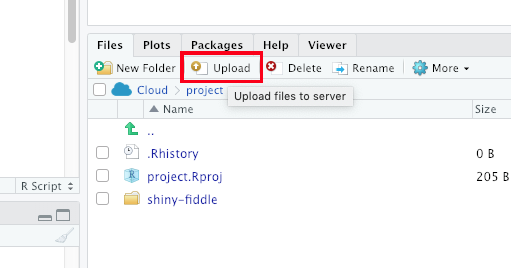
To open Data on Posit Cloud, you first need to Upload your file on this computer and to Import the data in R.
Open your Data as R Object (1)
Step 1: Upload your File
Step 2: Import your Data
Remember that .csv files are basically text files
Open your Data as R Object (2)
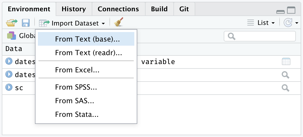
For early beginners on the Desktop version, directly open data with RStudio’s Import Dataset button.
If you see your data in the preview, you can click Import to create an object containing your data. A code will be executed, Copy and Paste the first line of this code in your R script. You will not have to do it manually once the code is in your script.
Open your Data as R Object (3)
To ensure code reproducibility, open data with the appropriate function (e.g., read.csv() for csv files).
The main argument of these functions is file which corresponds to the path to a file, followed by the name of the file and its extension:
# Incomplete pathmy_file_object <-read.csv("/path/to/my/file.csv")# Missing file extensionmy_file_object <-read.csv("C:/path/to/my/file")# Use of backward slashmy_file_object <-read.csv("C:\path\to\my\file.csv")
Live Demo
️ Your Turn!
Click on Upload to upload the “organisation_beta.csv” file on your Posit Cloud
Click on Import to import these data in R
Check that the data appears in the Environment pane. How many observations and variables does it have?
Copy the code that ran and paste it in your R script
05:00
5. Save Your Data
Save Your Data
Usually, only R Script files (.R) or Quarto files (.qmd) have to be saved as they allow the full replicability of transformations and results.
However, if you want to use the data that have been transformed, joined or pivoted, a function has to be used according to the type of export.
Save Your Data
The simplest export is a .csv file with the function write.csv(). It has two main arguments:
x which is the name of the object to save
file which is the name of the output file
Note: don’t forget the file extension in the argument file
# Saved in the current directorywrite.csv(x = my_file_object, file ="my_file_name.csv")write.csv(my_file_object, "my_file_name.csv")# Saved in the directory you preferwrite.csv(my_file_object, "C:/path/to/my/my_file_name.csv") # Windowswrite.csv(my_file_object, "/Users/path/to/my/my_file_name.csv") # Macos
️ Your Turn!
Save the data contained in the object “organisation_beta” in a new .csv file (give a different name than “organisation_beta.csv” else this document will be overwritten)
03:00
Become Expert in R
Plenty of free learning materials are available online:
If it’s not obvious, copy-paste the error in Google
2. Look at your object
str(ObjectName)
3. Look at the function
Documentation (F1 or ?)
4. GenAI
6. Linear Regression Models in R
Model and Equations
A model contains:
Only one Outcome Variable
One or more Predictor Variables of any type (categorical or continuous)
Main and/or Interaction Effects
Model and Equations
To evaluate their relationship with the outcome, each effect hypothesis is related with a coefficient called Estimate and represented with \(b\) as follows:
Testing for the significance of the effect means evaluating if this estimate \(b\) value is significantly different, higher or lower than 0 as hypothesised in \(H_a\) by the scientist.
Estimates and Linear Regression in R
The lm() function calculates each estimate and tests them against 0 for you.
lm() has only two arguments that you should care about: formula and data.
formula is the translation of the equation of the model
data is the name of the data frame object containing the variables.
Estimates and Linear Regression in R
Here is a generic example:
lm(formula = Outcome ~ Pred1 + Pred2, data = my_data_object)
Here is an example with organisation_beta.csv:
lm(formula = js_score ~ salary + perf, data = organisation_beta)
Mastering the Formula
lm() has only one difficulty, the formula. The formula is the direct translation of the equation tested but with its own representation:
The = sign is replaced by ~ (read “according to” or “by”)
Each predictor is added with the + sign
An interaction effect uses the symbol : instead of *
Mastering the Formula
Here are some generic equations and their conversion in formula:
\[Outcome = b_0 + b_1 Pred1 + b_2 Pred2 + e\]
lm(formula = Outcome ~ Pred1 + Pred2, data = my_data_object)
The next part provides a quick summary of the residuals (i.e., the \(e\) values),
Residuals:
      Min       1Q   Median       3Q      Max
 -2.04185 -0.49565  0.06529  0.61611  1.71635
This can be convenient as a quick check that the model is okay. Linear regression assumes that these residuals were normally distributed, with mean 0. In particular it’s worth quickly checking to see if the median is close to zero, and to see if the first quartile is about the same size as the third quartile. If they look badly off, there’s a good chance that the assumptions of regression are violated.
LM Summary
The next part of the R output looks at the coefficients of the regression model:
Each row in this table refers to one of the coefficients estimated in the regression model.
The first row is the intercept term, and the later ones look at each of the predictors. The columns give you all of the relevant information:
The first column is the actual estimate of b (e.g., -49.1865079 for the intercept, 0.0018837 for salary and -0.5946699 for gender).
The second column is the standard error estimate (SE).
The third column gives you the t-statistic.
Finally, the fourth column gives you the actual p value for each of these tests.
LM Summary
The only thing that the previous table doesn’t list is the degrees of freedom used in the t-test, which is always N−K−1 and is listed immediately below, in this line:
Residual standard error: 0.8854 on 17 degrees of freedom
LM Summary
The value of df=17 is equal to N−K−1, so that’s what we use for our t-tests. In the final part of the output we have the F-test and the R² values which assess the performance of the model as a whole
Multiple R-squared:  0.7613,    Adjusted R-squared:  0.7333
F-statistic: 27.12 on 2 and 17 DF,  p-value: 0.000005141
So in this case, the model performed significantly better than you’d expect by chance (F(2,17) = 27.12, p < 0.001), which isn’t all that surprising: the R² = 0.7333 value indicates that the regression model accounts for 73.3% of the variability in the outcome measure.
When we look back up at the t-tests for each of the individual coefficients, we have pretty strong evidence that salary has a significant effect.
Reporting Clean Results
To communicate about your statistical analyses in an academic report, the simplest method is to find the values in the summary() output and to copy-paste them in the text according to the format expected that we have seen in the previous lectures.
However, this task can be long, difficult and lead to human errors. Thankfully, R has additional packages that provide alternative functions to read linear regression models and communicate results.
Because there are too many packages, I will focus only on two additional packages: {performance} and {report}.
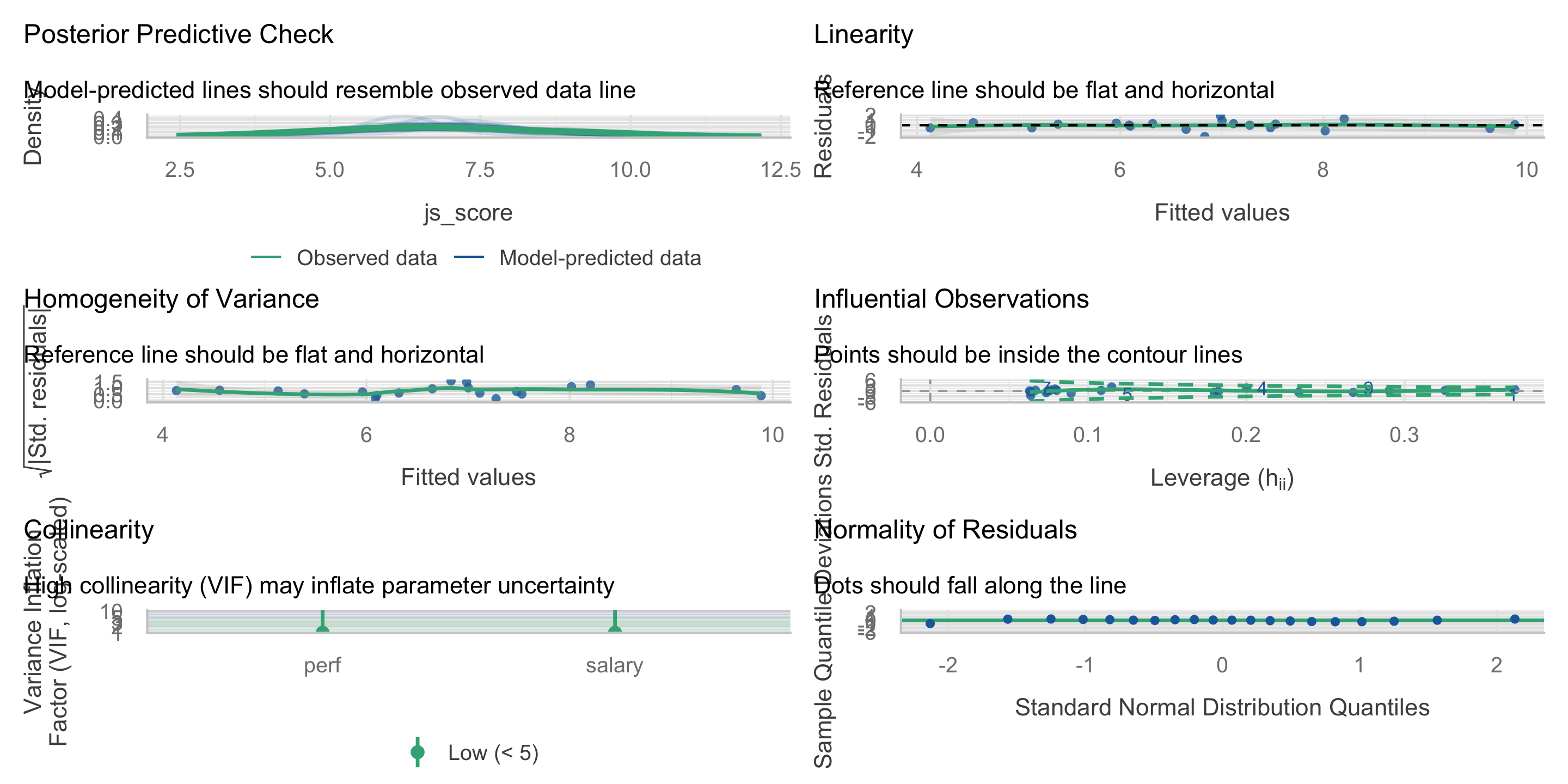
Assumption Check with {performance}
To install {performance} use the usual install.packages() function:
To install {report} use the usual install.packages() function:
install.packages("report")
The package {report} will print a text containing all the statistics already in sentences ready to be interpreted (see https://easystats.github.io/report/).
Automatic Results with {report}
To print the statistical analyses:
Load the package {report}
Create an object containing the output of the function lm()
Use this object as input of the function report() from the {report} package
Note: If used in a quarto document, the chunk containing report() has to include the chunk option results='asis'
We fitted a linear model (estimated using OLS) to predict js_score with salary and perf (formula: js_score ~ salary + perf). The model explains a statistically significant and substantial proportion of variance (R2 = 0.74, F(2, 17) = 24.16, p < .001, adj. R2 = 0.71). The model’s intercept, corresponding to salary = 0 and perf = 0, is at -49.49 (95% CI [-66.60, -32.37], t(17) = -6.10, p < .001). Within this model:
The effect of salary is statistically significant and positive (beta = 1.87e-03, 95% CI [1.30e-03, 2.44e-03], t(17) = 6.95, p < .001; Std. beta = 0.86, 95% CI [0.60, 1.13])
The effect of perf is statistically non-significant and positive (beta = 0.08, 95% CI [-0.15, 0.32], t(17) = 0.75, p = 0.465; Std. beta = 0.09, 95% CI [-0.17, 0.35])
Standardized parameters were obtained by fitting the model on a standardized version of the dataset. 95% Confidence Intervals (CIs) and p-values were computed using a Wald t-distribution approximation.
Live Demo
️ Your Turn!
In Posit Cloud, check the check_model() and report() output from the lm() function testing the following models: