MT611 - Quantitative Research Methods

class: center, middle, inverse, title-slide

.title[
# MT611 - Quantitative Research Methods
]
.subtitle[
## Lecture 8: Introduction to Quarto for Research
]
.author[
### Damien Dupré - Dublin City University
]

---

# Objectives

In this lecture, with Posit Cloud, we will see how to create **Quarto** files (.qmd) to embed text and code output and generate professional outputs.

#### What do I need to do before starting?

- Sign up for a free Posit cloud account
- https://posit.cloud/

#### Where can I find more resources?

- [Official Quarto Website](https://quarto.org/)
- [R for Data Science](https://r4ds.hadley.nz/quarto.html)
- [Appsilon](https://appsilon.com/r-quarto-tutorial/)
- [Making shareable documents with Quarto](https://openscapes.github.io/quarto-website-tutorial/)
- [Quarto 2hr webinar](https://jthomasmock.github.io/quarto-2hr-webinar/materials/01-intro-quarto.html)

---

# What is Quarto?

Quarto is an open-source scientific and technical publishing system that builds on standard markdown with features essential for scientific communication.

- Computations: Python, R, Julia, Observable JS
- Markdown: Pandoc flavored markdown with many enhancements
- Output: Documents, presentations, websites, books, blogs

See https://quarto.org for more details

The Goal is to create a document that is all-in-one

- Documents that include source code for their production
- Notebook AND plain-text flavors
- Programmatic automation and reproducibility

---

# Two Sides of Quarto Files

.pull-left[
### On the editor side...

- Write text in markdown
- Insert code using R or Python
- Write "metadata" with YAML
]

.pull-right[
### On the output side...

- Output to HTML
- Output to PDF
- Output to Word
- Many other variations too
]

Try it by yourself!

---
class: title-slide, middle

## Your turn!

In your Posit Cloud:

1/ Create a new Quarto document: `File > New File > Quarto Document`

2/ A popup will appear, untick **"Use visual markdown editor"**

3/ Leave everything else as default and click `Create`

4/ If a warning appears, click `Install` on the message to install the {rmarkdown} package

![](https://raw.githubusercontent.com/damien-dupre/img/main/rmarkdown_warning.png)

5/ Click the blue arrow `Render` and save the document as `report.qmd`

---

# Simple Example

---

# Simple Example

.pull-left[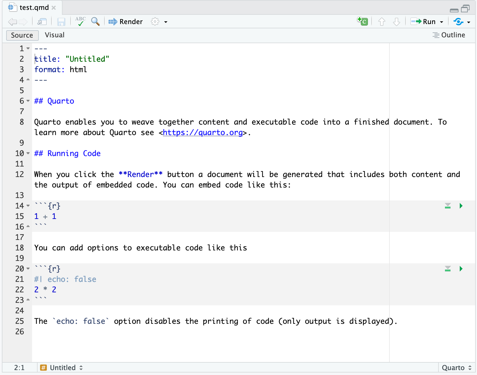
![](https://raw.githubusercontent.com/damien-dupre/img/main/quarto_default.png)
]

.pull-right[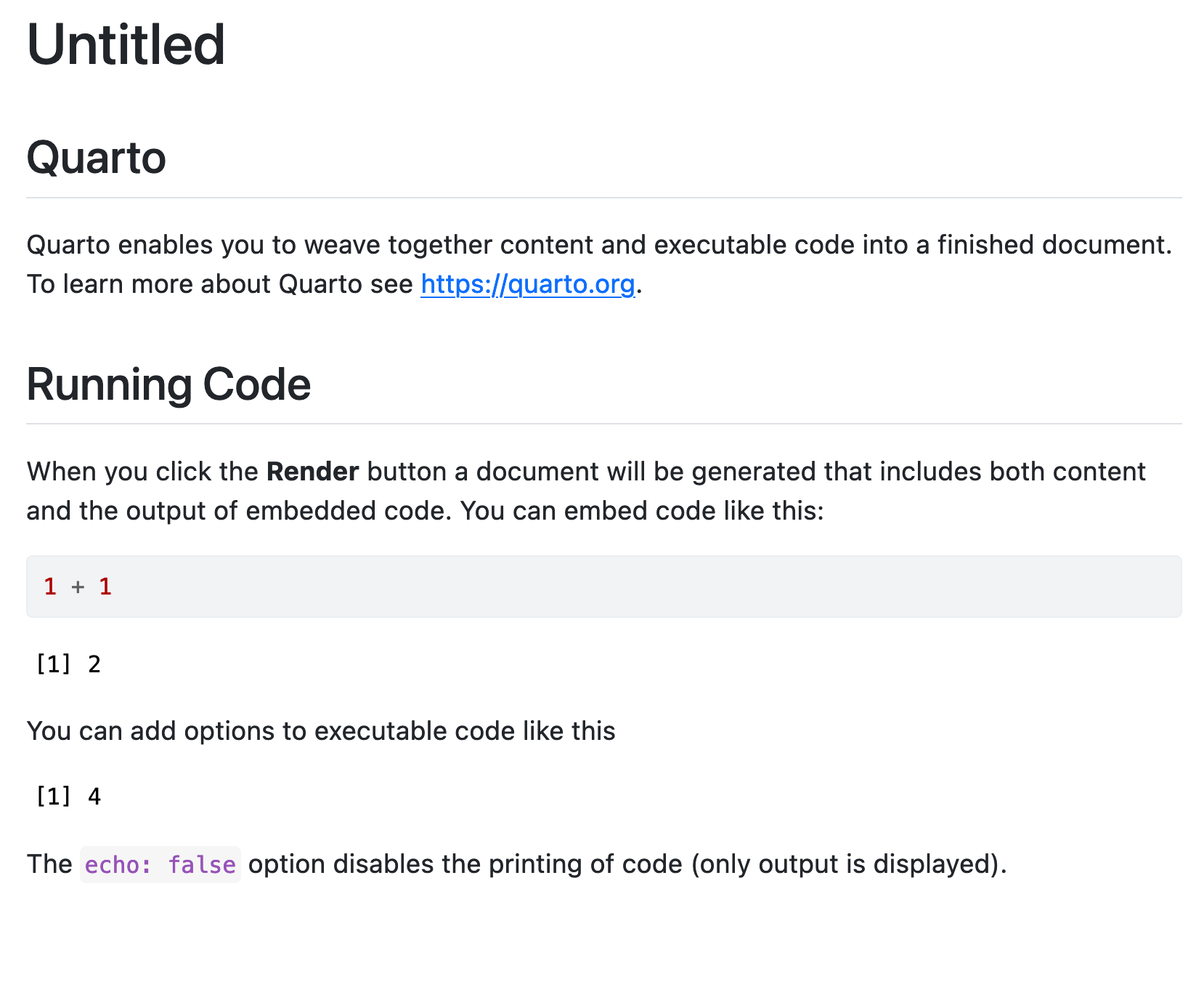
![](https://raw.githubusercontent.com/damien-dupre/img/main/quarto_create.png)
]

---

# Quarto Structure

Quarto files have 3 different types of content:

#### 1. The YAML

Displayed between two series of `---` signs, it corresponds to the metadata shown in the header of the output file (e.g., title, author, date, ...) and the type of output (e.g., pdf, html, doc, ...)

#### 2. The Text

Written in Markdown style (i.e., text without formatting), it is used as core description in the output document

#### 3. The Code

Inserted in the Quarto inside "chunks", the code is processed when creating the output and can display figures and tables

---

# The "YAML"

---

# The Markdown Text

---

# The R Code

---

# Create the Output File

.pull-left[
To generate the output file:

1/ Go to `File > Render Document` (a  Use the `Render` shortcut icon is also displayed in the menu bar)

<kbd>![](https://quarto.org/docs/get-started/hello/images/rstudio-render-button.png)</kbd>

![](https://quarto.org/docs/get-started/hello/images/rstudio-render.png)

2/ Give a name to your document, click `OK`, and voila!
]

.pull-right[
<img src="https://raw.githubusercontent.com/damien-dupre/img/main/quarto_create.png" width="100%" />
]

---

# Quarto Editor vs Output

.pull-left[
![](https://raw.githubusercontent.com/damien-dupre/img/main/quarto_default.png)
]

.pull-right[
![](https://raw.githubusercontent.com/damien-dupre/img/main/quarto_create.png)
]

---
class: inverse, mline, center, middle

# 1. The YAML

---

# Output HTML

### Simple

```
---
format: html
---
```

### Default

```
---
title: "My First Quarto Document"
format: html
date: "99/99/9999"
---
```

### Elaborated

```
---
title: "My First Quarto Document"
subtitle: "My Subtitle"
author: "Damien Dupre"
date: "99/99/9999"
format: html
---
```

---

# Execute Code

Quarto can use R or Python to execute code:

- R code is executed natively with the `{knitr}` engine
- Quarto can _also_ use the `Jupyter` engine to execute Julia, Python, or other languages that Jupyter supports

.pull-left[
If R code is found first will default to `knitr`

```yaml
---
format: html
---
```

Or can force using `knitr` if you're mixing R/Python content or if your first code chunk is not R.

```yaml
---
format: html
engine: knitr
---
```
]

.pull-right[
You can specify Jupyter to use defaults:

```yaml
---
engine: jupyter
---
```

Or a specific Python version

```yaml
---
engine: python3
---
```
]

---

# Execute Code

Quarto also introduces some of these as options for `execute:` in YAML, for similar concepts in other languages.

```yaml
---
format: html
execute:
  echo: false
  warning: false
  message: false
---
```

---
class: inverse, mline, center, middle

# 2. Markdown Style

---

# Emphasising Text

.pull-left[
<br><br>
### What you type...
<br>
```

this is *italics*

this is **bold**

this is ***bold italics***
```
]
--
.pull-right[
<br><br>
### What you get...
<br>

this is *italics*

this is **bold**

this is ***bold italics***
]

---

# Creating Lists

.pull-left[
<br><br>
### What you type...
<br>
```
- unnumbered lists
- look like this

1. numbered lists
2. look like this
```
]
--
.pull-right[
<br><br>
### What you get...
<br>

- unnumbered lists
- look like this

1. numbered lists
2. look like this
]

---

# Creating Headings

.pull-left[
<br><br>
### What you type...
<br>
```
# Level 1 heading
## Level 2 heading
### Level 3 heading

```
]
--
.pull-right[
<br><br>
### What you get...
<br>

## Level 1 heading
### Level 2 heading
#### Level 3 heading
]

---

# LaTeX Equations

.pull-left[
<br><br>
### What you type...
<br>
```
$$
JS_i = b_0 + b_1 Salary_i + b_2 Perf_i + e_i
$$

$$
e_{i} \sim \mathcal{N}(0, \sigma_{i})
$$

```
]
--
.pull-right[
<br><br>
### What you get...
<br>

$$
JS_i = b_0 + b_1 Salary_i + b_2 Perf_i + e_i
$$

$$
e_i \sim \mathcal{N}(0, \sigma_i)
$$

]

---

# Markdown Example

.pull-left[

**Example of a markdown document...**

```
## Introduction

Welcome to my **awesome** class. You 
will learn all kinds of useful things 
about Quarto.

- Markdown is simple
- You can add R code
- You can add $\LaTeX$ inline
- You can add LaTex equations:

$$y=ax+b$$

```
]

.pull-right[

**Here's what the output looks like...**

## Introduction
<br>
Welcome to my **awesome** class. You will learn 
all kinds of useful things about Quarto.

- Markdown is simple
- You can add R code
- You can add `$\LaTeX$` inline
- You can add LaTeX equations:

`$$y=ax+b$$`

]

---
class: title-slide, middle

## Your turn!

In Posit Cloud, with the file that you have previously created:

1/ Remove all content except the YAML

2/ Modify the YAML to include:

```yaml
---
format: html
execute:
  echo: false
  warning: false
  message: false
---
```

3/ Write a sentence about your emotions (positive and negative) triggered by R, use `*` and `**` to highlight some part of your text in italic and bold

4/ Add a section title with `##` and a subsection title with `###`

5/ Click "Render" once finished

---

class: inverse, mline, center, middle

# 3. The R Code Chunks

---

# Anatomy of a Code Chunk

````markdown
```{r}
#| label: organisation-beta-lm
#| echo: false
model <- lm(formula = js_score ~ salary + perf, data = organisation_beta)
```
````

- Has 3x backticks on each end ` ``` ` 
- Place engine (`r`) between curly braces `{r}`  
- Place options underneath, behind the `#|` (hashpipe): `#| option1: value`

---

# First Code Chunk

In the first code chunk, will be added all the __actions that will be applied to the following chunks__ (e.g., code option, library used, data downloaded, ...).

````markdown
```{r}
#| label: setup
#| include: false

# libraries
library(tidyverse)
  
# data
organisation_beta <- read_csv("/cloud/project/organisation_beta.csv")
```

````

---

# Code Chunk Options

Chunk output can be customized with hashpipe options (i.e., arguments set after the `#|`). Above, we use 1 argument:

- `#| include: false` prevents code and results from appearing in the finished file. Quarto still runs the code in the chunk, and the results can be used by other chunks.

Additional options can be turned on only for one chunk:

- `#| results: asis` will display the output of the code as regular text

See the **[Quarto Reference Guide](https://quarto.org/docs/reference/cells/cells-knitr.html)** for a complete list of chunk options.

---

# Figures in the Output Document

As long as the package {tidyverse} is loaded and the data object created in the first setup chunk, then a __ggplot visualisation can be used in a separated chunk__:

.small[
````markdown
---
title: "Untitled"
output: html
execute:
  echo: false
  warning: false
  message: false
---

```{r}
#| label: setup
#| include: false

library(tidyverse)

organisation_beta <- read_csv("/cloud/project/organisation_beta.csv")
```

# My Section Title

My text followed by my figure.

```{r}
ggplot(organisation_beta) +
  aes(salary, js_score) +
  geom_point()
```
````
]

---

# Working with Code

To display the output of your code in the final document, just include your code in a chunk:

````markdown
```{r}
lm(formula = js_score ~ salary + perf, data = organisation_beta)
```
````

```
## 
## Call:
## lm(formula = js_score ~ salary + perf, data = organisation_beta)
## 
## Coefficients:
## (Intercept)       salary         perf  
##   -49.48511      0.00187      0.08285
```

---

# Working with Code

Remember, when the code results in creating an object, while the object is created, no output is printed in the final document:

````markdown
```{r}
model <- lm(formula = js_score ~ salary + perf, data = organisation_beta)
```
````

---

# Working with Code

To create an object and print your code in the same chunk, the name of the object has to be included in the chunk. This will print the content of the object:

````markdown
```{r}
model <- lm(formula = js_score ~ salary + perf, data = organisation_beta)
  
model
```
````

```
## 
## Call:
## lm(formula = js_score ~ salary + perf, data = organisation_beta)
## 
## Coefficients:
## (Intercept)       salary         perf  
##   -49.48511      0.00187      0.08285
```

---

# Visualisation Specific Options

Some chunk options are specific to visualisations outputs:

- fig-cap: "caption of the figure"
- fig-height: 5
- fig-width: 5

Note, the default unit for height and width is inches.

````markdown
```{r}
#| fig-cap: "caption of the figure"
#| fig-height: 5
#| fig-width: 5

ggplot(organisation_beta) +
  aes(salary, js_score) +
  geom_point()
```
````

![Example Caption](lecture_8_files/figure-html/unnamed-chunk-17-1.png)

---
class: title-slide, middle

## Live Demo

---
class: title-slide, middle

## Your turn!

In your **report.qmd** document:

1/ **Create a first code chunk** called `setup`. In this chunk, load the `{tidyverse}` and `{report}` packages and create your data object with the following code:

```markdown
organisation_beta <- read_csv("/cloud/project/organisation_beta.csv")
```

3/ **Create a second code chunk**. In this chunk, run the following linear regression and add `#| results: asis` in its options:

```markdown
lm_js <- lm(formula = js_score ~ salary + perf, data = organisation_beta)

report(lm_js)
```

---
class: title-slide, middle

## Your turn!

4/ Create a third code chunk. In this chunk, include the following visualisation:

```markdown
ggplot(organisation_beta) +
  aes(salary, js_score) +
  geom_point() +
  geom_smooth(method = "lm") +
  theme_bw() +
  labs(
    x = "Employee Salary (Eur)",
    y = "Employee's Job Satisfaction"
  )
```

5/ Render the default document obtained to observe its structure

---
class: inverse, mline, center, middle

# 4. Gallery

---

# Professional Websites

---

# Books

---

# Slide Decks

---

# CV

---

# Academic Papers

---
class: inverse, mline, center, middle

# 5. Quarto Journal Templates

---

# Quarto Journal Templates

The Quarto team has developed several Journal formats and made them available within the [quarto-journals GitHub organization](https://github.com/quarto-journals/). These formats include the following Journal/Publisher:

- Association of Computing Machinery
- American Chemical Society
- American Geophysical Union
- Biophysical journal
- Elsevier Journals
- American Statistical Association
- Journal of Statistical Software

Many more formats will be added over time.

The quarto use template command can be used to create an article from one these formats from the terminal (and not the console). For example:

```
quarto use template quarto-journals/acm
quarto use template quarto-journals/acs
quarto use template quarto-journals/agu
quarto use template quarto-journals/biophysical-journal
quarto use template quarto-journals/elsevier
quarto use template quarto-journals/jasa
quarto use template quarto-journals/jss
quarto use template quarto-journals/plos
```

---
class: title-slide, middle

## Live Demo

---
class: title-slide, middle

## Your turn!

In your Posit Cloud:

1/ Create a new quarto-journals document using one of the following template from the terminal:

Say `Y` when asked if you trust the authors of this template and choose a directory name of your choice.

2/ Render the default .qmd document obtained to observe its structure

---
class: title-slide, middle

## Your turn!

In this new .qmd document:

1/ Remove everything except the YAML

2/ Create a first `setup` chunk. In this chunk, load the `{tidyverse}` and `{report}` packages and create your data object with the following code:

```markdown
organisation_beta <- read_csv("/cloud/project/organisation_beta.csv")
```

3/ Create a second code chunk. In this chunk, run the following linear regression and add `#| results: asis` in its options:

```markdown
lm_js <- lm(formula = js_score ~ salary + perf, data = organisation_beta)

report(lm_js)
```

---
class: title-slide, middle

## Your turn!

4/ Create a third code chunk. In this chunk, include the following visualisation:

5/ Render the default document obtained to observe its structure

---
class: inverse, mline, center, middle

# 6. Quarto Website Templates

---

# Quarto Websites

Quarto Websites are a convenient way to publish groups of documents. Documents published as part of a website share navigational elements, rendering options, and visual style.

Website navigation can be provided through a global navbar, a sidebar with links, or a combination of both for sites that have multiple levels of content. You can also enable full text search for websites.

![](https://www.paulbarrs.com/wp-content/uploads/2017/09/painful.jpg)

---
class: title-slide, middle

## Your turn!

1/ In the Terminal window, run the following instructions:

```markdown
quarto create project website mysite
```

and

```markdown
quarto render mysite
```

2/ Go to any `.qmd` file and click **Render**

Note: If you proceed these instructions from your desktop, you need to install quarto first: https://quarto.org/
]

---

# Quarto Websites

```markdown
quarto create project website mysite
```

Creates a new website project from the Terminal. This website project is initiated by a folder called `mysite` located on the root of your terminal.

The folder contains only 4 files:
- `_quarto.yml` is a yaml file, it design the overall style and the navbar
- `index.qmd` is a quarto file, it corresponds to the homepage
- `about.qmd` is another quarto file which is displayed when about is clicked on the navbar
- `styles.css` is for additional style not defined in `_quarto.yml`

Improve your Website:

- Navigation instructions here: https://quarto.org/docs/websites/website-navigation.html
- Option instructions here: https://quarto.org/docs/reference/projects/websites.html

---

# Quarto Websites

```markdown
quarto render mysite
```

These commands are used to render the website by converting all the `.qmd` files to `.html` files stored in a `_site` folder.

The website preview will open in a new web browser. As you edit and save `index.qmd` (or other files like `about.qmd`) the preview is automatically updated.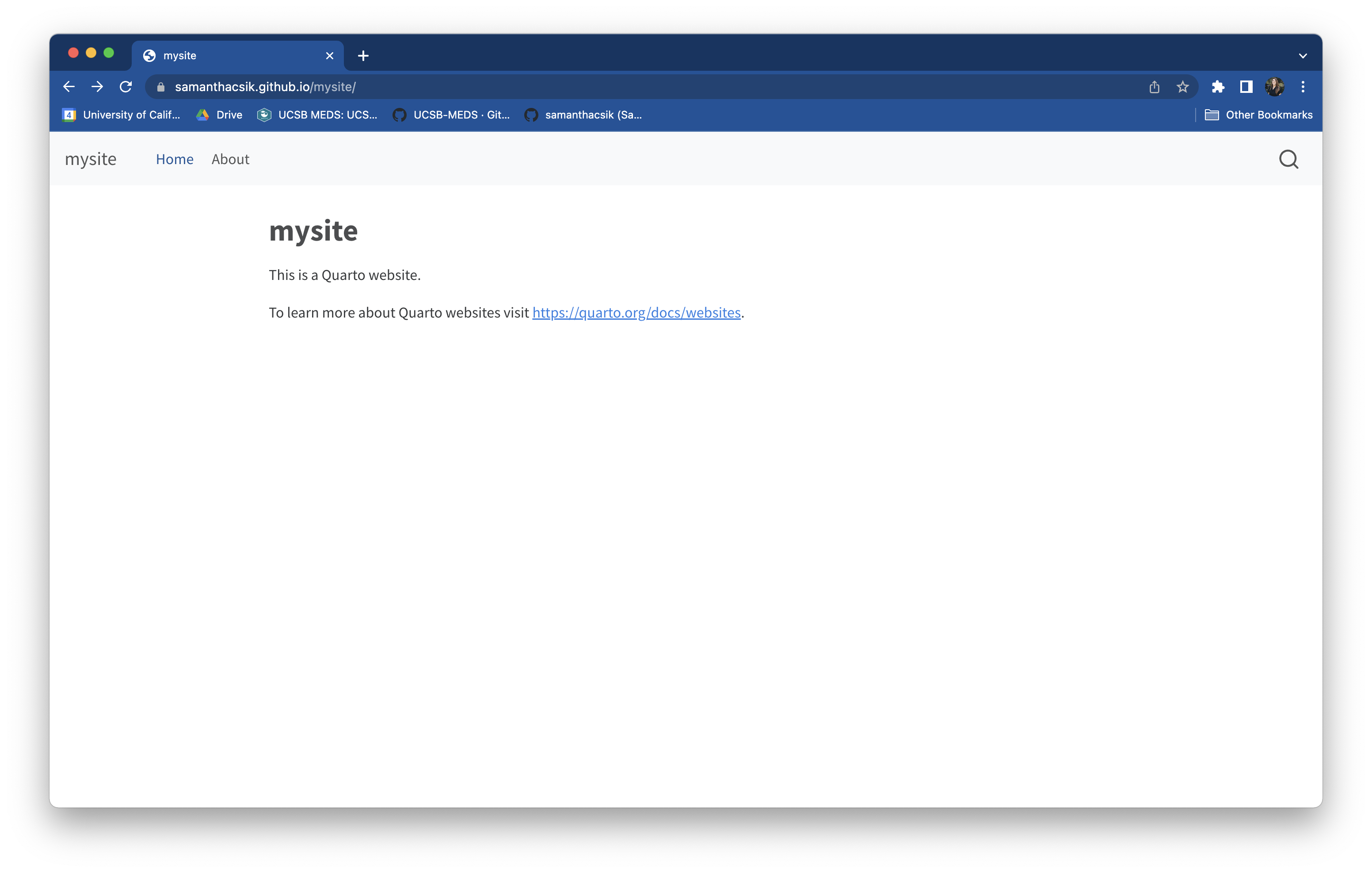

![](https://ucsb-meds.github.io/creating-quarto-websites/media/rendered_site.png)

---
class: title-slide, middle

## Your turn!

1/ Open the first file created `report.qmd`, change `format: pdf` to `format: html` and save it in the folder `mysite`

2/ Open the file `_quarto.yml` and modify it as follow:

```markdown
website:
  title: "Mysite"
  navbar:
    left:
      - href: index.qmd
        text: Home
      - about.qmd
      - report.qmd
```

4/ In the same Terminal window, run the following instructions:

```markdown
quarto render mysite
```

5/ Go to any `.qmd` file and click **Render**

---
class: inverse, mline, center, middle

# 7. Publish this website on GitHub

---

# Render the Website docs Folder

In the `_quarto.yml` file, simply **change the output directory folder** to a folder named `docs` as follow:

```markdown
project:
  type: website
  output-dir: docs
```

Then render the website:

```markdown
quarto render mysite
```

.pull-left[
Your website default folder should look like that →

Note: the old folder `_site` will not be used any more and is now useless.
]

.pull-right[
<img src="https://raw.githubusercontent.com/damien-dupre/img/main/mysite_docs.png" width="80%" />
]

---

# Add a .nojekyll File

Add a `.nojekyll` file to the root of your repository that tells GitHub Pages not to do additional processing of your published site using Jekyll (the GitHub default site generation tool):

You can create an empty text file by yourself or you can download this `nojekyll` file here:
<button class="btn btn-default" onclick="fetch('data:text/plain;base64,').then(res => res.blob()).then(blob => {
      const downloadURL = window.URL.createObjectURL(blob);
      const a = document.createElement('a');
      a.style.display = 'none'; // Hide the link
      document.body.appendChild(a);
      a.href = downloadURL;
      a.download = 'nojekyll.';
      a.click();
      window.URL.revokeObjectURL(downloadURL);
      document.body.removeChild(a);
      return false;
    });"><i class="fa fa-save"></i> Click here to download nojekyll</button>

---

# Upload your Files to GitHub

Just drag and drop all the files in GitHub at once like this:

---
class: title-slide, middle

## Your turn!

.pull-left[
1/ **Change the output directory folder** to a folder named `docs` in the `_quarto.yml` file:

```markdown
project:
  type: website
  output-dir: docs
```

Then, preview or render the website

```markdown
quarto render mysite
```

2/ **Upload and commit all the files contained in the website folder** on your GitHub repository, not the website folder itself.
]

.pull-right[
3/ **Upload and commit a nojekyll file** that tells GitHub to not run its default html website processing

You can download this `nojekyll` file here:

<button class="btn btn-default" onclick="fetch('data:text/plain;base64,').then(res => res.blob()).then(blob => {
      const downloadURL = window.URL.createObjectURL(blob);
      const a = document.createElement('a');
      a.style.display = 'none'; // Hide the link
      document.body.appendChild(a);
      a.href = downloadURL;
      a.download = 'nojekyll.';
      a.click();
      window.URL.revokeObjectURL(downloadURL);
      document.body.removeChild(a);
      return false;
    });"><i class="fa fa-save"></i> Click here to download nojekyll</button>

4/ Finally, in **GitHub**, click **Settings** -> **Pages** choose:
- `main` branch
- `/docs` folder
- and Save
]

---
class: inverse, mline, left, middle

# Thanks for your attention and don't hesitate to ask if you have any questions!

[<svg aria-hidden="true" role="img" viewBox="0 0 512 512" style="height:1em;width:1em;vertical-align:-0.125em;margin-left:auto;margin-right:auto;font-size:inherit;fill:currentColor;overflow:visible;position:relative;"><path d="M459.37 151.716c.325 4.548.325 9.097.325 13.645 0 138.72-105.583 298.558-298.558 298.558-59.452 0-114.68-17.219-161.137-47.106 8.447.974 16.568 1.299 25.34 1.299 49.055 0 94.213-16.568 130.274-44.832-46.132-.975-84.792-31.188-98.112-72.772 6.498.974 12.995 1.624 19.818 1.624 9.421 0 18.843-1.3 27.614-3.573-48.081-9.747-84.143-51.98-84.143-102.985v-1.299c13.969 7.797 30.214 12.67 47.431 13.319-28.264-18.843-46.781-51.005-46.781-87.391 0-19.492 5.197-37.36 14.294-52.954 51.655 63.675 129.3 105.258 216.365 109.807-1.624-7.797-2.599-15.918-2.599-24.04 0-57.828 46.782-104.934 104.934-104.934 30.213 0 57.502 12.67 76.67 33.137 23.715-4.548 46.456-13.32 66.599-25.34-7.798 24.366-24.366 44.833-46.132 57.827 21.117-2.273 41.584-8.122 60.426-16.243-14.292 20.791-32.161 39.308-52.628 54.253z"/></svg> @damien_dupre](http://twitter.com/damien_dupre)  
[<svg aria-hidden="true" role="img" viewBox="0 0 496 512" style="height:1em;width:0.97em;vertical-align:-0.125em;margin-left:auto;margin-right:auto;font-size:inherit;fill:currentColor;overflow:visible;position:relative;"><path d="M165.9 397.4c0 2-2.3 3.6-5.2 3.6-3.3.3-5.6-1.3-5.6-3.6 0-2 2.3-3.6 5.2-3.6 3-.3 5.6 1.3 5.6 3.6zm-31.1-4.5c-.7 2 1.3 4.3 4.3 4.9 2.6 1 5.6 0 6.2-2s-1.3-4.3-4.3-5.2c-2.6-.7-5.5.3-6.2 2.3zm44.2-1.7c-2.9.7-4.9 2.6-4.6 4.9.3 2 2.9 3.3 5.9 2.6 2.9-.7 4.9-2.6 4.6-4.6-.3-1.9-3-3.2-5.9-2.9zM244.8 8C106.1 8 0 113.3 0 252c0 110.9 69.8 205.8 169.5 239.2 12.8 2.3 17.3-5.6 17.3-12.1 0-6.2-.3-40.4-.3-61.4 0 0-70 15-84.7-29.8 0 0-11.4-29.1-27.8-36.6 0 0-22.9-15.7 1.6-15.4 0 0 24.9 2 38.6 25.8 21.9 38.6 58.6 27.5 72.9 20.9 2.3-16 8.8-27.1 16-33.7-55.9-6.2-112.3-14.3-112.3-110.5 0-27.5 7.6-41.3 23.6-58.9-2.6-6.5-11.1-33.3 2.6-67.9 20.9-6.5 69 27 69 27 20-5.6 41.5-8.5 62.8-8.5s42.8 2.9 62.8 8.5c0 0 48.1-33.6 69-27 13.7 34.7 5.2 61.4 2.6 67.9 16 17.7 25.8 31.5 25.8 58.9 0 96.5-58.9 104.2-114.8 110.5 9.2 7.9 17 22.9 17 46.4 0 33.7-.3 75.4-.3 83.6 0 6.5 4.6 14.4 17.3 12.1C428.2 457.8 496 362.9 496 252 496 113.3 383.5 8 244.8 8zM97.2 352.9c-1.3 1-1 3.3.7 5.2 1.6 1.6 3.9 2.3 5.2 1 1.3-1 1-3.3-.7-5.2-1.6-1.6-3.9-2.3-5.2-1zm-10.8-8.1c-.7 1.3.3 2.9 2.3 3.9 1.6 1 3.6.7 4.3-.7.7-1.3-.3-2.9-2.3-3.9-2-.6-3.6-.3-4.3.7zm32.4 35.6c-1.6 1.3-1 4.3 1.3 6.2 2.3 2.3 5.2 2.6 6.5 1 1.3-1.3.7-4.3-1.3-6.2-2.2-2.3-5.2-2.6-6.5-1zm-11.4-14.7c-1.6 1-1.6 3.6 0 5.9 1.6 2.3 4.3 3.3 5.6 2.3 1.6-1.3 1.6-3.9 0-6.2-1.4-2.3-4-3.3-5.6-2z"/></svg> @damien-dupre](http://github.com/damien-dupre)  
[<svg aria-hidden="true" role="img" viewBox="0 0 640 512" style="height:1em;width:1.25em;vertical-align:-0.125em;margin-left:auto;margin-right:auto;font-size:inherit;fill:currentColor;overflow:visible;position:relative;"><path d="M579.8 267.7c56.5-56.5 56.5-148 0-204.5c-50-50-128.8-56.5-186.3-15.4l-1.6 1.1c-14.4 10.3-17.7 30.3-7.4 44.6s30.3 17.7 44.6 7.4l1.6-1.1c32.1-22.9 76-19.3 103.8 8.6c31.5 31.5 31.5 82.5 0 114L422.3 334.8c-31.5 31.5-82.5 31.5-114 0c-27.9-27.9-31.5-71.8-8.6-103.8l1.1-1.6c10.3-14.4 6.9-34.4-7.4-44.6s-34.4-6.9-44.6 7.4l-1.1 1.6C206.5 251.2 213 330 263 380c56.5 56.5 148 56.5 204.5 0L579.8 267.7zM60.2 244.3c-56.5 56.5-56.5 148 0 204.5c50 50 128.8 56.5 186.3 15.4l1.6-1.1c14.4-10.3 17.7-30.3 7.4-44.6s-30.3-17.7-44.6-7.4l-1.6 1.1c-32.1 22.9-76 19.3-103.8-8.6C74 372 74 321 105.5 289.5L217.7 177.2c31.5-31.5 82.5-31.5 114 0c27.9 27.9 31.5 71.8 8.6 103.9l-1.1 1.6c-10.3 14.4-6.9 34.4 7.4 44.6s34.4 6.9 44.6-7.4l1.1-1.6C433.5 260.8 427 182 377 132c-56.5-56.5-148-56.5-204.5 0L60.2 244.3z"/></svg> damien-datasci-blog.netlify.app](https://damien-datasci-blog.netlify.app)  
[<svg aria-hidden="true" role="img" viewBox="0 0 512 512" style="height:1em;width:1em;vertical-align:-0.125em;margin-left:auto;margin-right:auto;font-size:inherit;fill:currentColor;overflow:visible;position:relative;"><path d="M16.1 260.2c-22.6 12.9-20.5 47.3 3.6 57.3L160 376V479.3c0 18.1 14.6 32.7 32.7 32.7c9.7 0 18.9-4.3 25.1-11.8l62-74.3 123.9 51.6c18.9 7.9 40.8-4.5 43.9-24.7l64-416c1.9-12.1-3.4-24.3-13.5-31.2s-23.3-7.5-34-1.4l-448 256zm52.1 25.5L409.7 90.6 190.1 336l1.2 1L68.2 285.7zM403.3 425.4L236.7 355.9 450.8 116.6 403.3 425.4z"/></svg> damien.dupre@dcu.ie](mailto:damien.dupre@dcu.ie)