02:00
Identifying Correct or Incorrect Emotion Recognition from Facial Expression Time Series using
Objectives
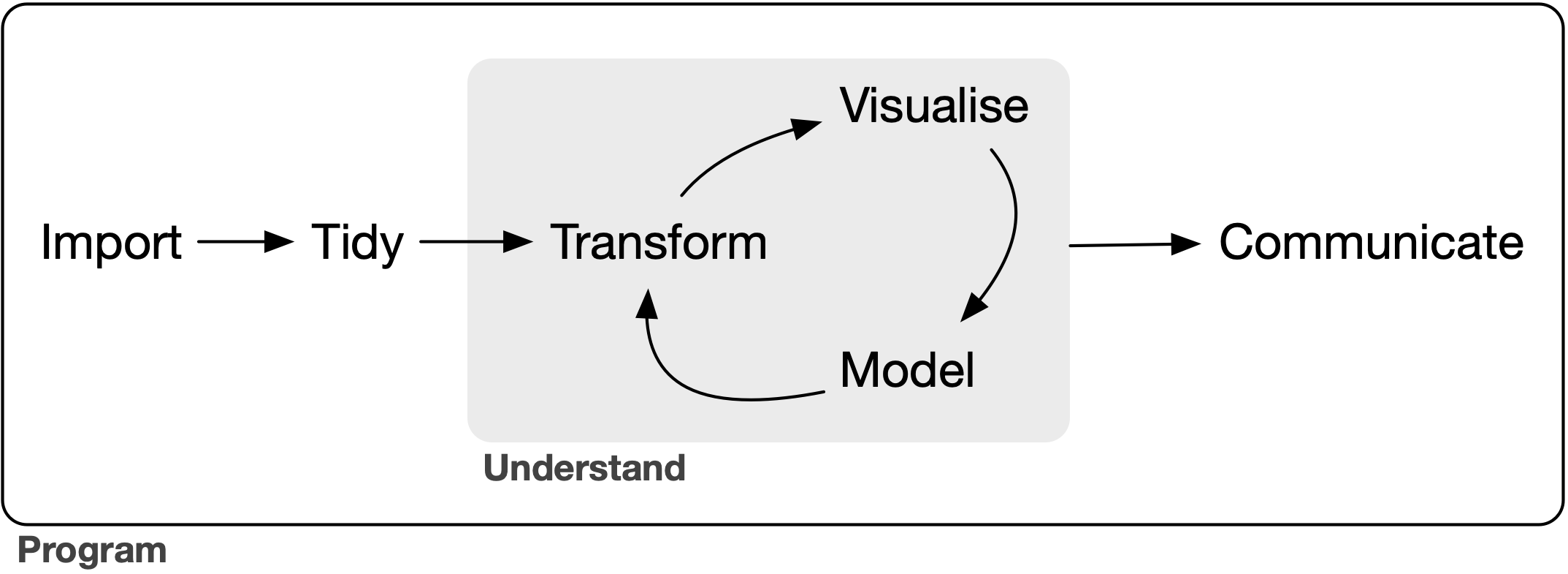
- Import, Tidy and Transform
- Visualise
- Model
- Communicate
🛠️ Now, it’s Your Turn!
- In your browser, sign up or log in at https://posit.cloud
- Click on New Project and choose New Project from Git Repository
- Enter
https://github.com/damien-dupre/cere2025_workshopwhen prompted for the repository URL

Single Recording
Let’s visualise a single video:
list_file <- unique(df_tidy_long$file)

df_tidy_long |>
  filter(file == list_file[3]) |>
  ggplot() +
  aes(
    x = frame,
    y = recognition,
    colour = emotion
  ) +
  geom_line(linewidth = 2) +
  theme_bw() +
  theme(legend.position = "bottom") +
  scale_y_continuous(limits = c(0, 1)) +
  scale_color_brewer(palette = "Dark2")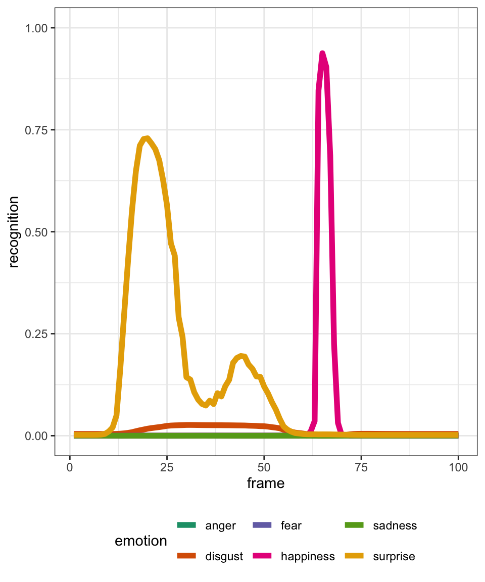
All Recordings for 1 Task
Let’s visualise recordings for one instruction task:
list_task <- unique(df_tidy_long$instruction)

df_tidy_long |>
  filter(instruction == list_task[3]) |>
  ggplot() +
  aes(
    x = frame,
    y = recognition,
    group = ppt,
    colour = emotion
  ) +
  geom_line(linewidth = 1, alpha = 0.2) +
  facet_grid(emotion ~ ., switch = "x") +
  theme_bw() +
  theme(legend.position = "bottom") +
  scale_y_continuous(breaks = c(0, 0.5, 1)) +
  scale_color_brewer(palette = "Dark2") +
  guides(colour = "none")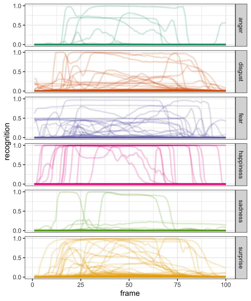
Model
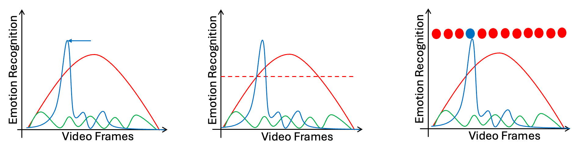
Here is a visual representation of each method applied to a special case in which all methods return the same emotion recognised.
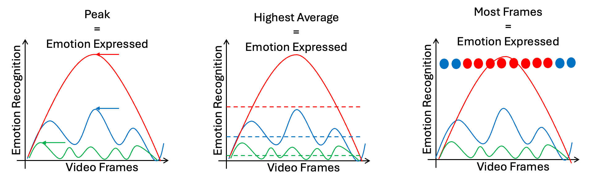
Model
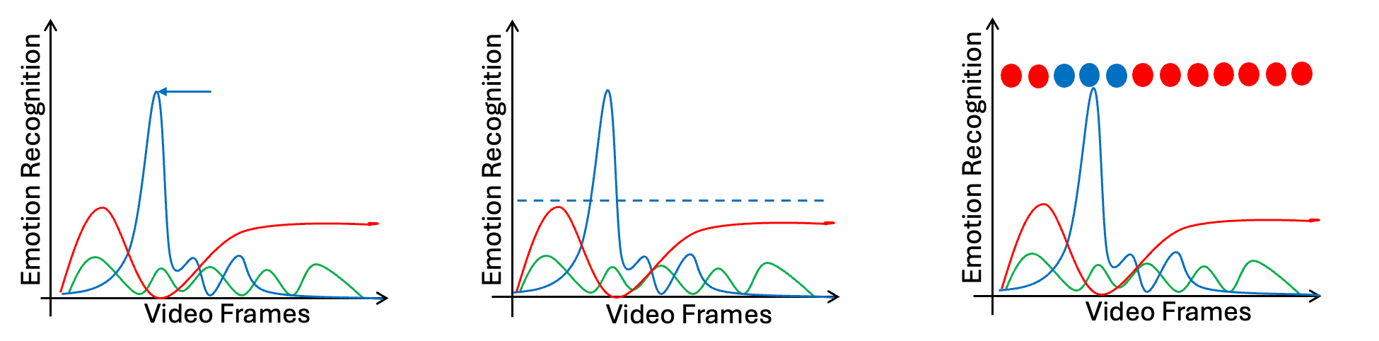
However, some cases are returning different results:
Effects Visualisation
Let’s calculate the average congruency by instruction task and by method with a basic visualisation:
df_congruency |>
  group_by(method, instruction) |>
  summarise(mean_se(congruency)) |>
  ggplot() +
  aes(
    x = instruction,
    y = y,
    ymin = ymin,
    ymax = ymax,
    fill = method,
    shape = method
  ) +
  geom_errorbar(position = position_dodge(width = 0.8)) +
  geom_point(
    size = 4,
    position = position_dodge(width = 0.8)
  ) +
  theme_bw() +
  theme(legend.position = "bottom")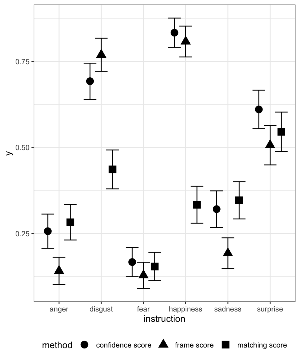
Effects Visualisation
Here is the same visualisation but with more customisations:
df_congruency |>
  group_by(method, instruction) |>
  summarise(mean_se(congruency)) |>
  ggplot() +
  aes(
    x = fct_reorder(instruction, y, .fun = "mean"),
    y = y,
    ymin = ymin,
    ymax = ymax,
    fill = method,
    shape = method
  ) +
  ggstats::geom_stripped_cols() +
  geom_errorbar(width = 0, position = position_dodge(width = 0.8)) +
  geom_point(stroke = 0, size = 4, position = position_dodge(width = 0.8)) +
  scale_y_continuous("Congruence between instruction and recognition", limits = c(0, 1), labels = scales::percent) +
  scale_x_discrete("") +
  scale_fill_brewer("Method", palette = "Dark2") +
  scale_shape_manual("Method", values = c(21, 22, 23, 24)) +
  guides(
    shape = guide_legend(reverse = TRUE, position = "inside"),
    fill = guide_legend(reverse = TRUE, position = "inside")
  ) +
  theme_bw() +
  theme(
    text = element_text(size = 12),
    axis.text.x = element_text(size = 14),
    axis.text.y = element_text(size = 14),
    axis.line.y = element_blank(),
    legend.title = element_text(hjust = 0.5),
    legend.position.inside = c(0.8, 0.2),
    legend.background = element_rect(fill = "grey80")
  ) +
coord_flip(ylim = c(0, 1)) 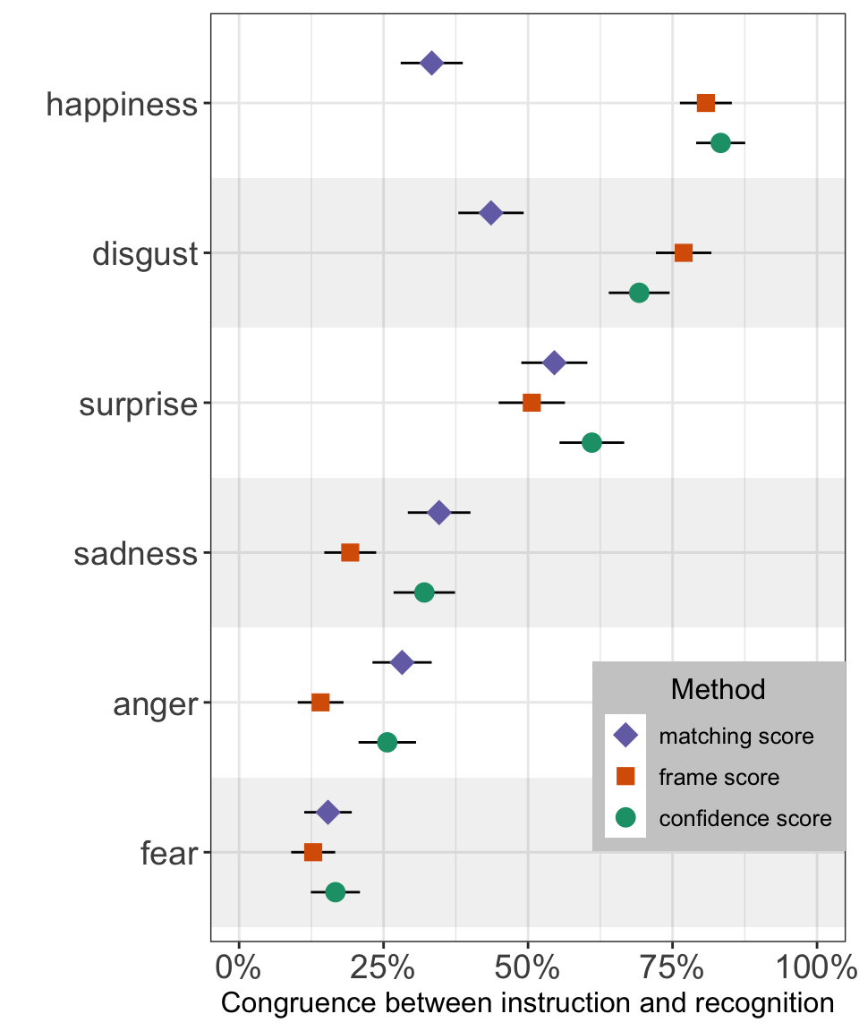
On Theory
- Each participant was instructed by a psychologist to gradually portray the six basic emotions in distinct sequences, their expression are not genuine
- Low congruence scores does not necessarily indicate an issue with the participants, it could be due to recognition system limitations


Thanks for your attention and don’t hesitate to ask if you have any questions!
@damien_dupre
@damien-dupre
https://damien-dupre.github.io
damien.dupre@dcu.ie