05:00
STA1005 - Quantitative Research Methods
Lecture 8: Introduction to Quarto for Research
️ Your Turn!
In your Posit Cloud:
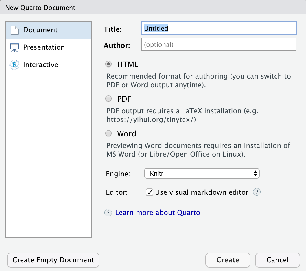
- Create a new Quarto document:
File > New File > Quarto Document - A popup will appear, untick “Use visual markdown editor”
- Leave everything else as default and click
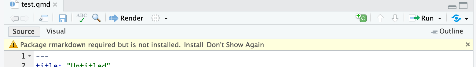
Create - If a warning appears, click
Installon the message to install the {rmarkdown} package
- Click the blue arrow
Renderand save the document asreport.qmd
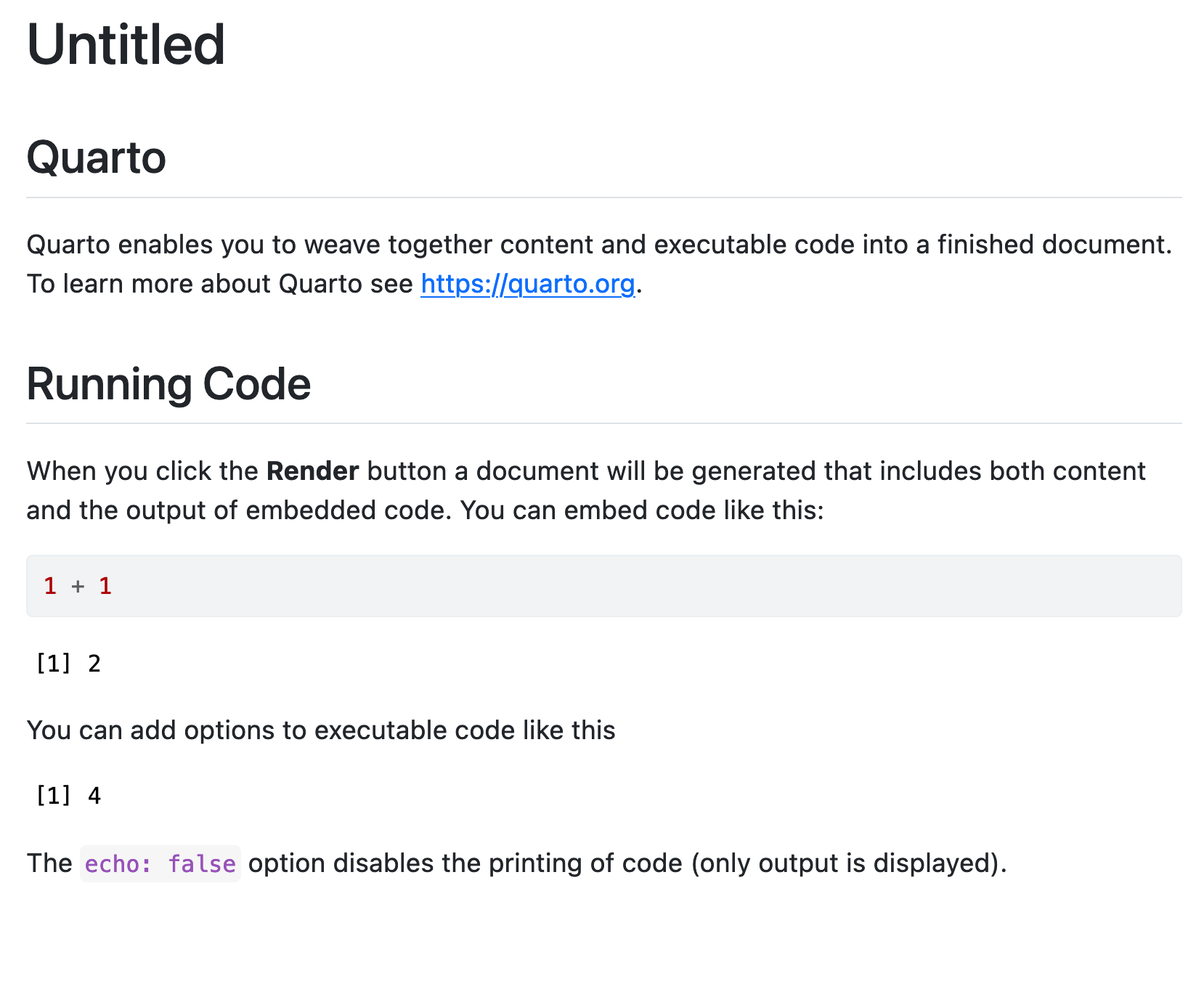
Simple Example
Simple Example
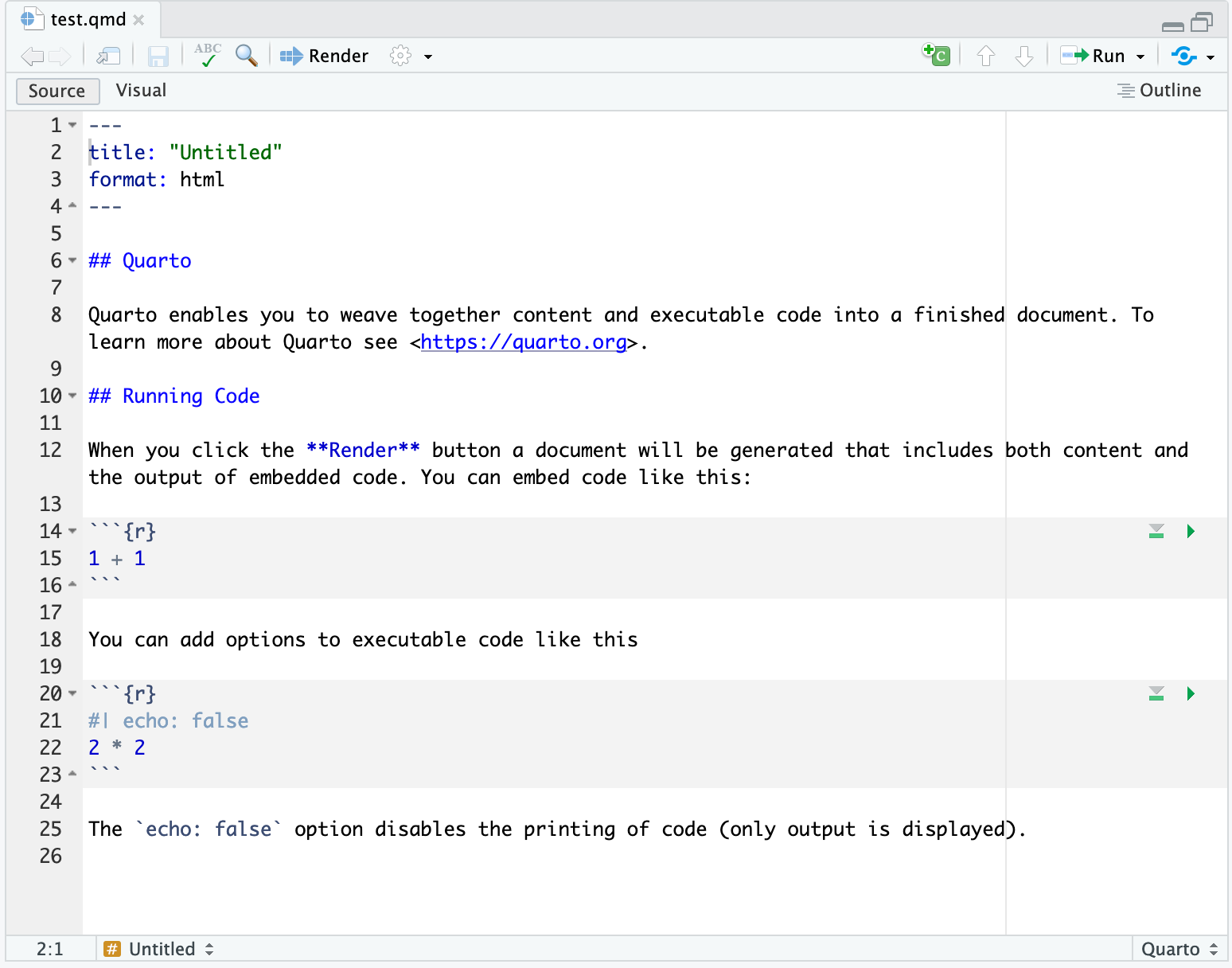
The “YAML”
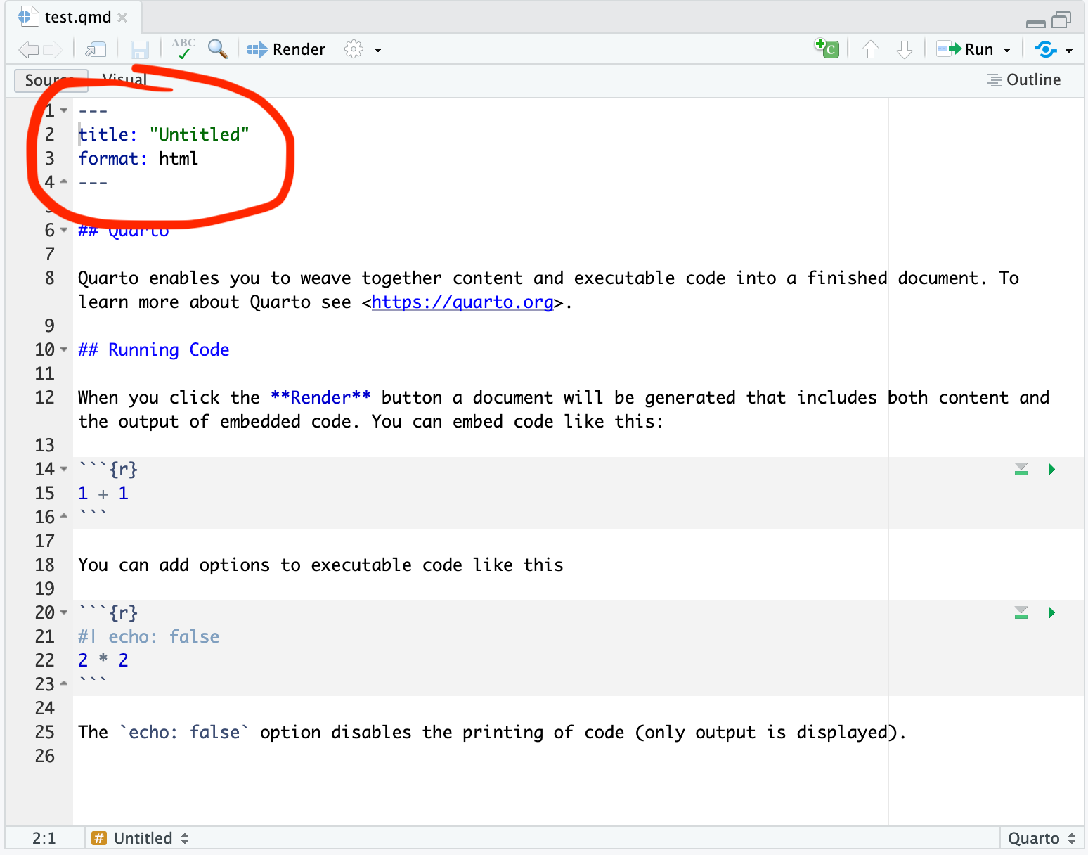
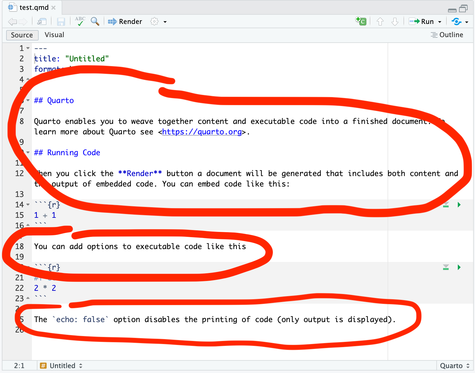
The Markdown Text
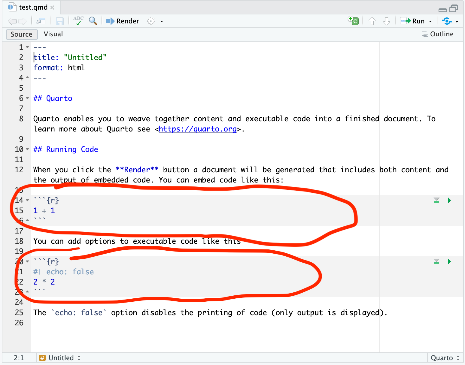
The R Code
Create the Output File
To generate the output file:
- Go to
File > Render Document(aRendershortcut icon is also displayed in the menu bar)

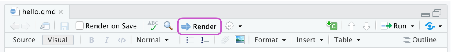
- Give a name to your document, click
OK, and voila!
Quarto Editor vs Output
Visualisation Specific Options
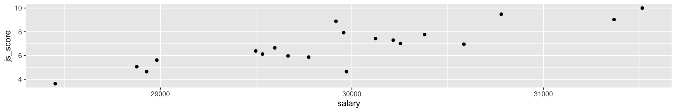
Example Caption
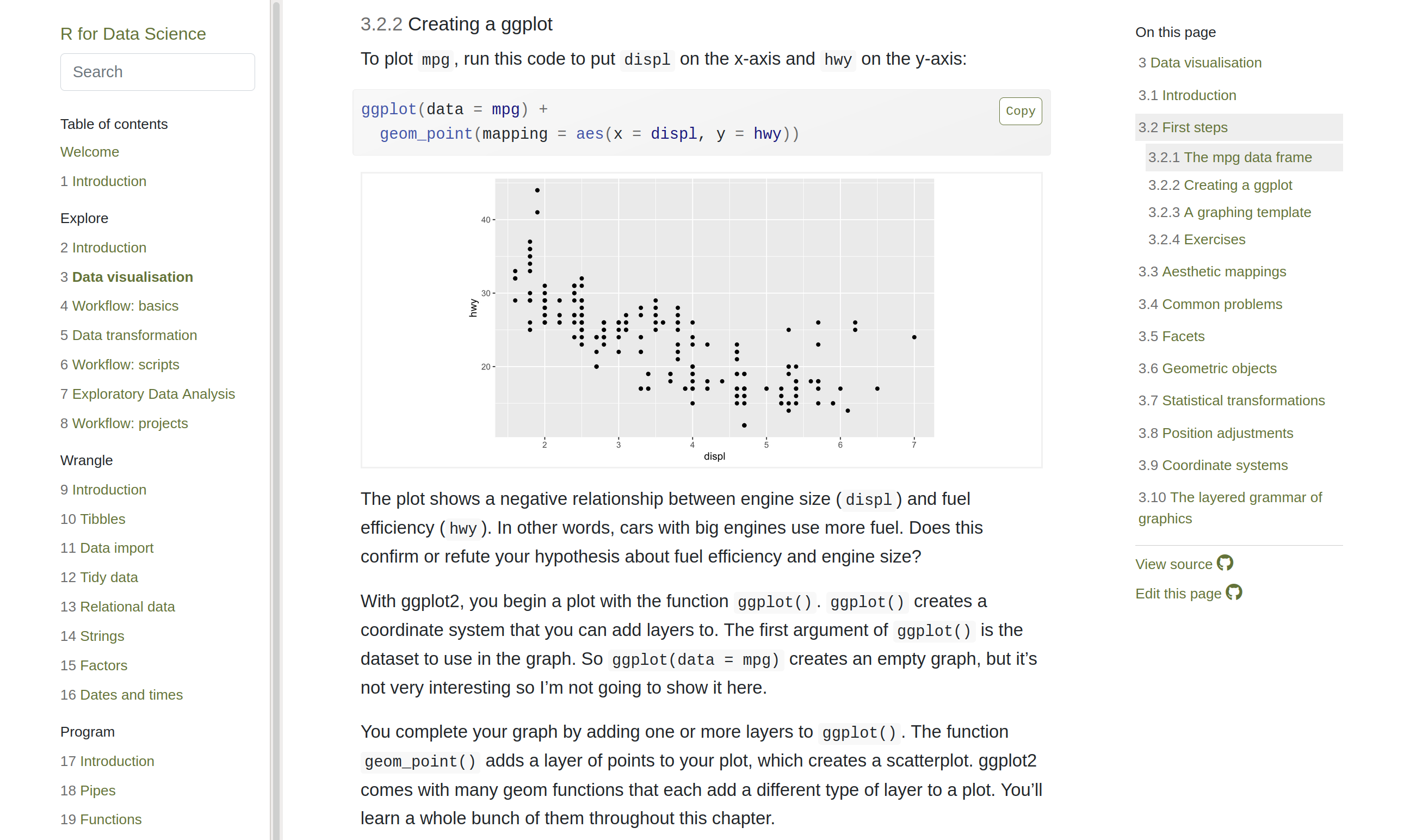
Professional Websites

Books
Slide Decks

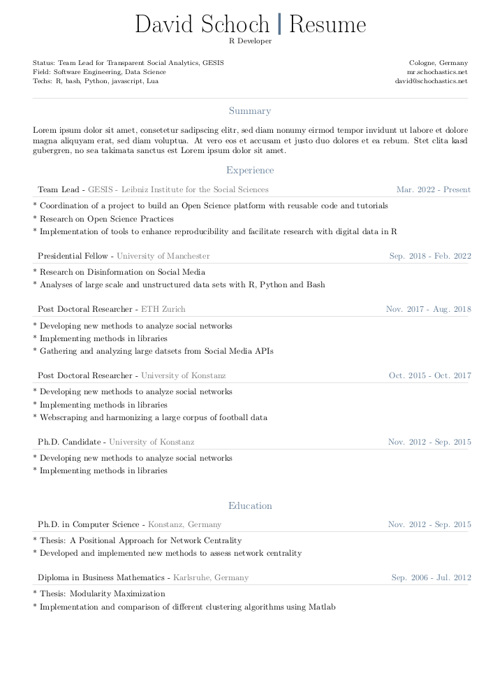
CV
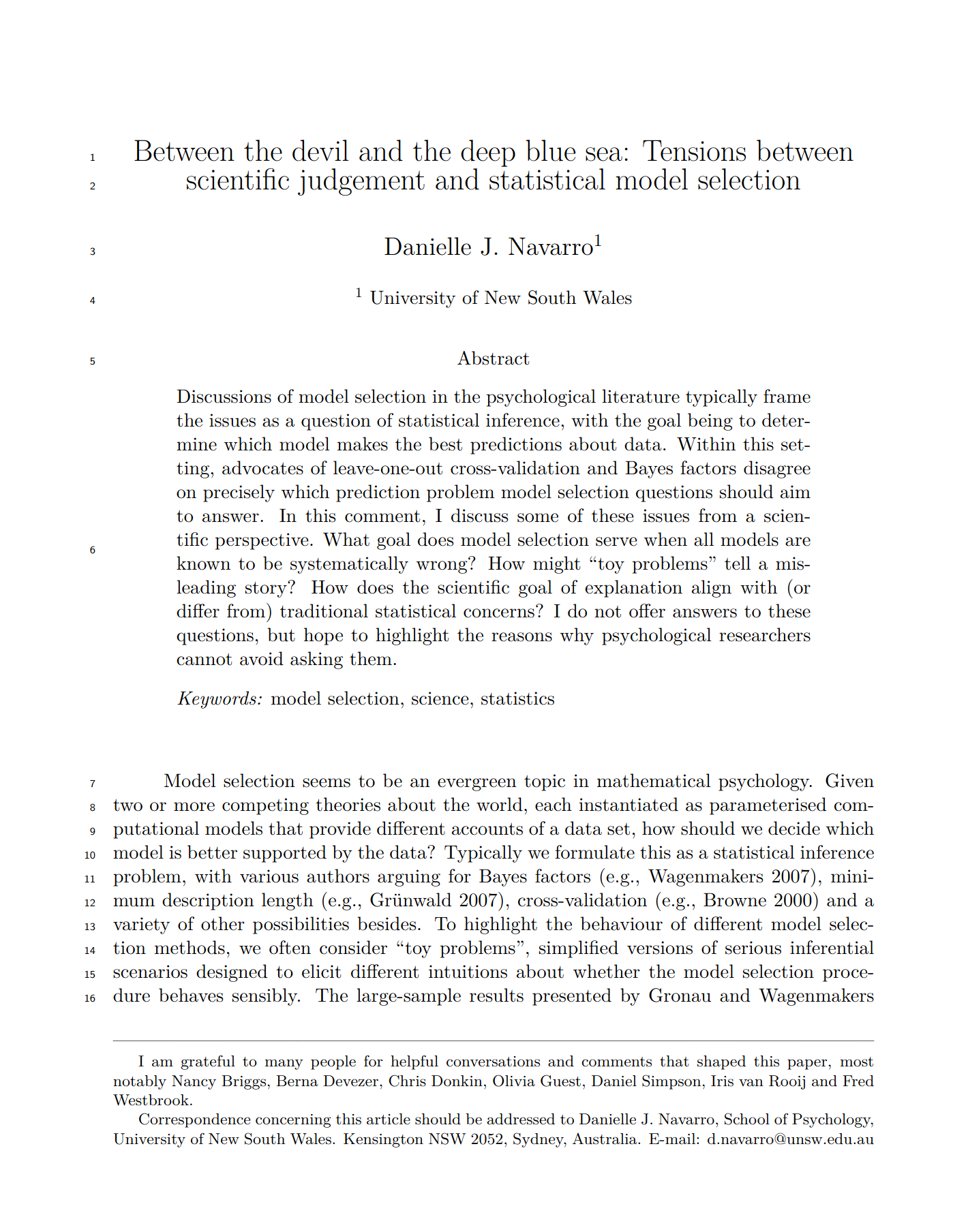
Academic Papers
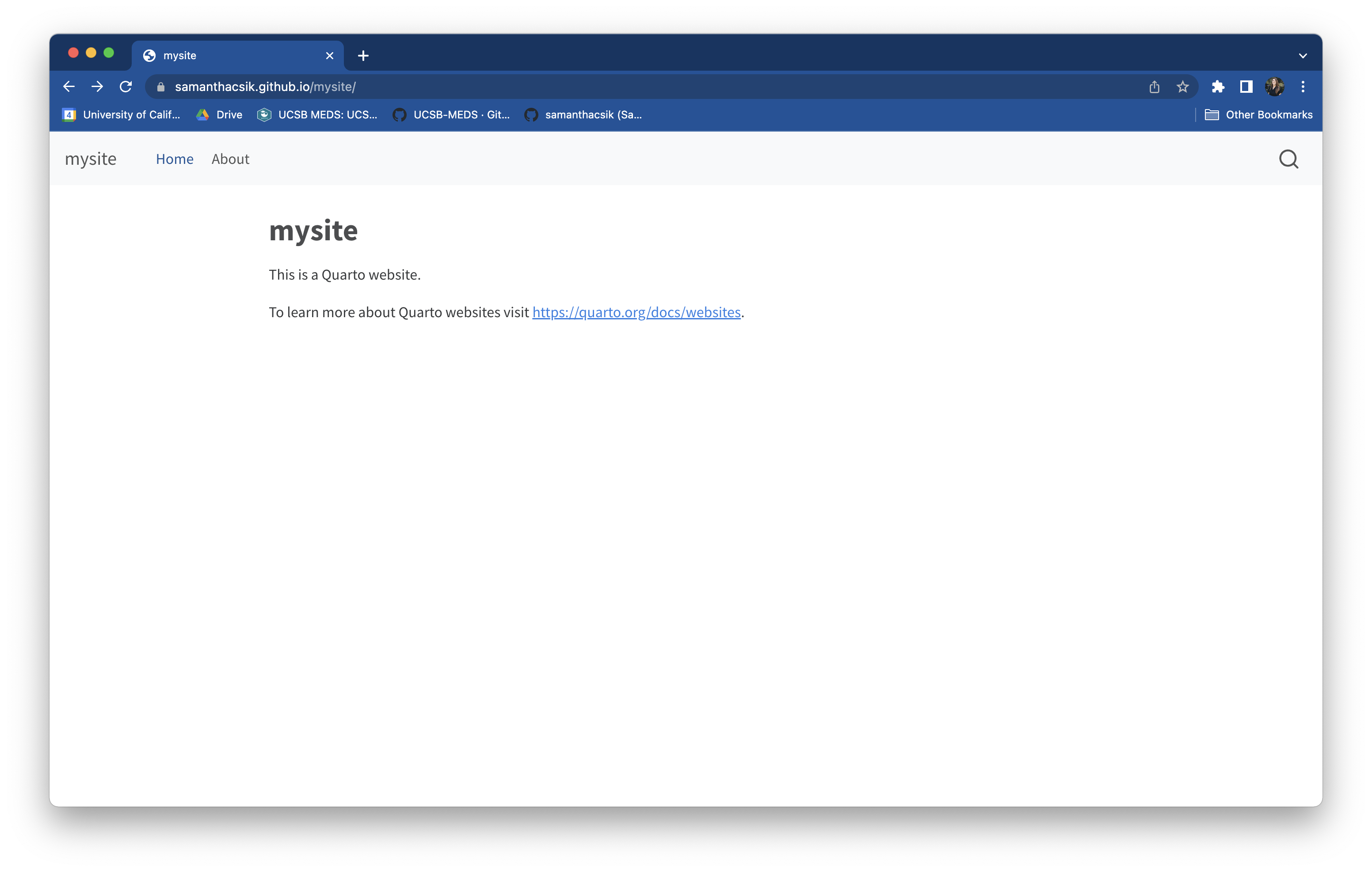
Quarto Websites
Quarto Websites are a convenient way to publish groups of documents. Documents published as part of a website share navigational elements, rendering options, and visual style.
Website navigation can be provided through a global navbar, a sidebar with links, or a combination of both for sites that have multiple levels of content. You can also enable full text search for websites.

Quarto Websites
These commands are used to render the website by converting all the .qmd files to .html files stored in a _site folder.
The website preview will open in a new web browser. As you edit and save index.qmd (or other files like about.qmd) the preview is automatically updated.
Demonstration
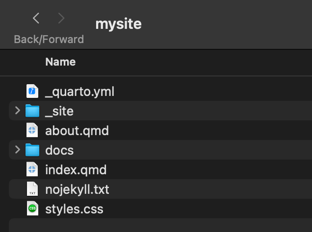
Your website default folder should look like that →
Note
The old folder _site will not be used any more and is now useless.
Demonstration
In GitHub, just drag and drop all the files at once like this:
Finally, click Settings -> Pages choose:
mainbranch/docsfolder- and Save
Thanks for your attention
and don’t hesitate to ask if you have any questions!