| employee | gender | js_score |
|---|---|---|
| 1 | female | 5.057311 |
| 2 | male | 6.642440 |
| 3 | male | 6.119694 |
| 4 | female | 9.482198 |
| 5 | female | 8.883347 |
| 6 | female | 7.015606 |
| 7 | male | 4.633738 |
| 8 | female | 7.919998 |
| 9 | male | 9.028004 |
| 10 | female | 5.860449 |
| 11 | male | 10.000000 |
| 12 | male | 3.617721 |
| 13 | male | 6.948510 |
| 14 | male | 7.429012 |
| 15 | female | 7.292992 |
| 16 | male | 7.765043 |
| 17 | male | 6.380634 |
| 18 | male | 5.962925 |
| 19 | male | 5.607226 |
| 20 | female | 4.635931 |
STA1005 - Quantitative Research Methods
Lecture 5: Categories in the General Linear Model
Vocabulary
Specific tests are available for certain type of hypothesis such as T-test or ANOVA but as they are special cases of Linear Regressions, their importance is limited (see Jonas Kristoffer Lindeløv’s blog post: Common statistical tests are linear models).

Hypotheses with Categorical Predictors
We will have a deep dive in the processing of Categorical predictor variables with linear regressions:
- How to analyse a predictor with only 2 categories?
- How to analyse a predictor with more than 2 categories?
Example of Categorical Coding
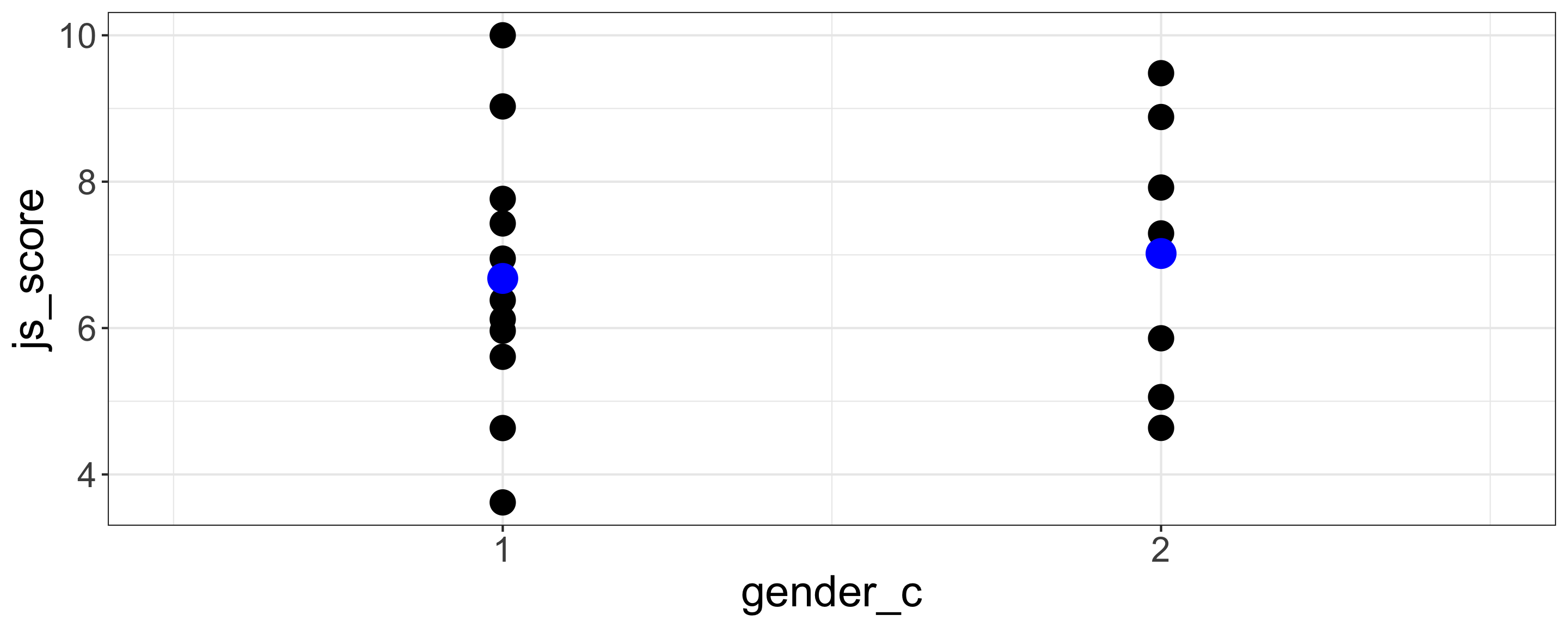
Using a Categorical variable having 2 category, e.g., comparing female vs. male …
… is the same as comparing female coded 1 and male coded 2
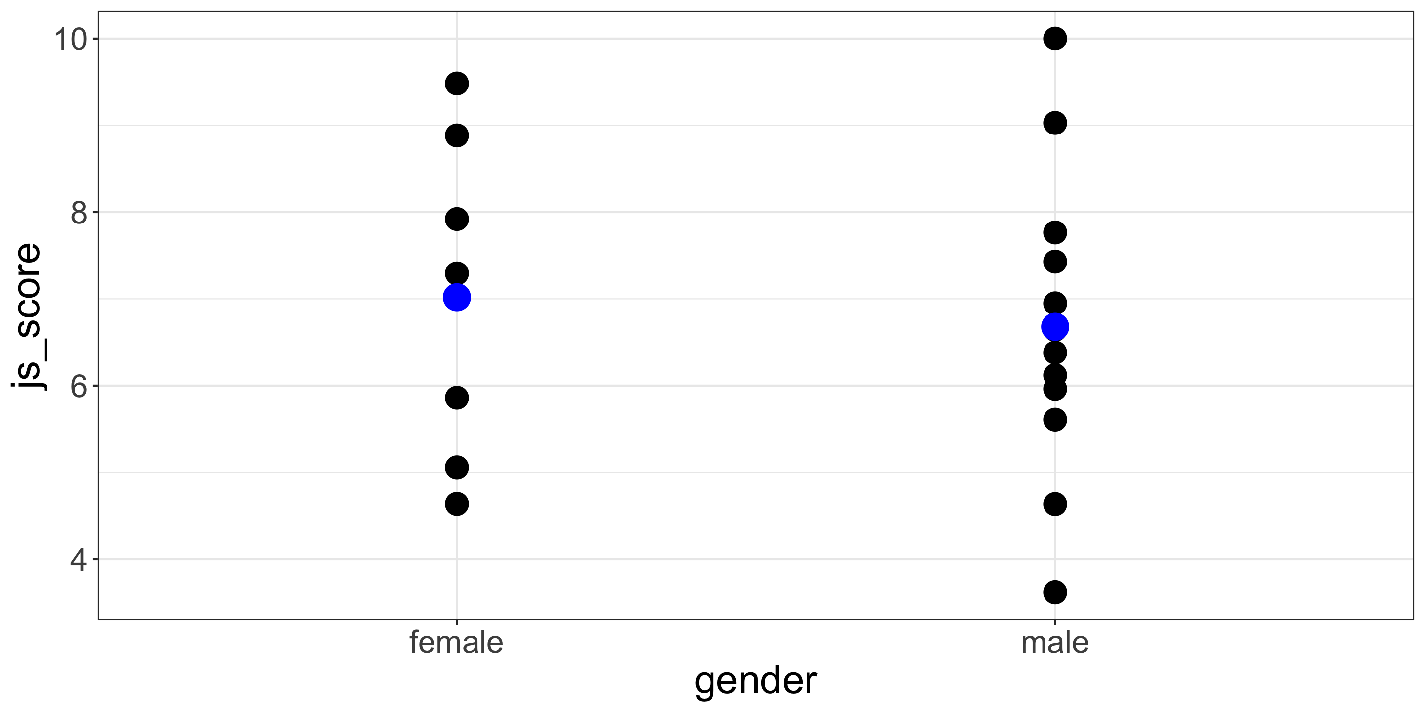
Categorical Coding in Linear Regression
Default
Female = 1 and Male = 2
| term | estimate | std.error | statistic | p.value |
|---|---|---|---|---|
| (Intercept) | 7.36 | 1.34 | 5.50 | <0.001 |
| gender_c | -0.34 | 0.80 | -0.43 | 0.675 |
Manual
Male = 1 and Female = 2
| term | estimate | std.error | statistic | p.value |
|---|---|---|---|---|
| (Intercept) | 6.34 | 1.19 | 5.34 | <0.001 |
| gender_c | 0.34 | 0.80 | 0.43 | 0.675 |
Categorical Predictor with 2 Categories
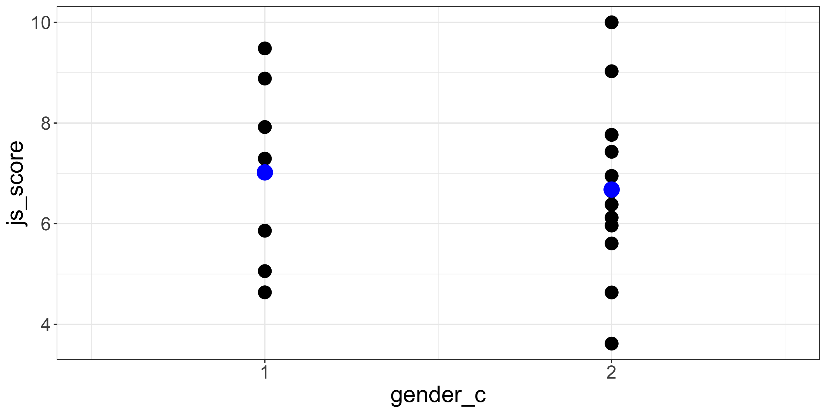
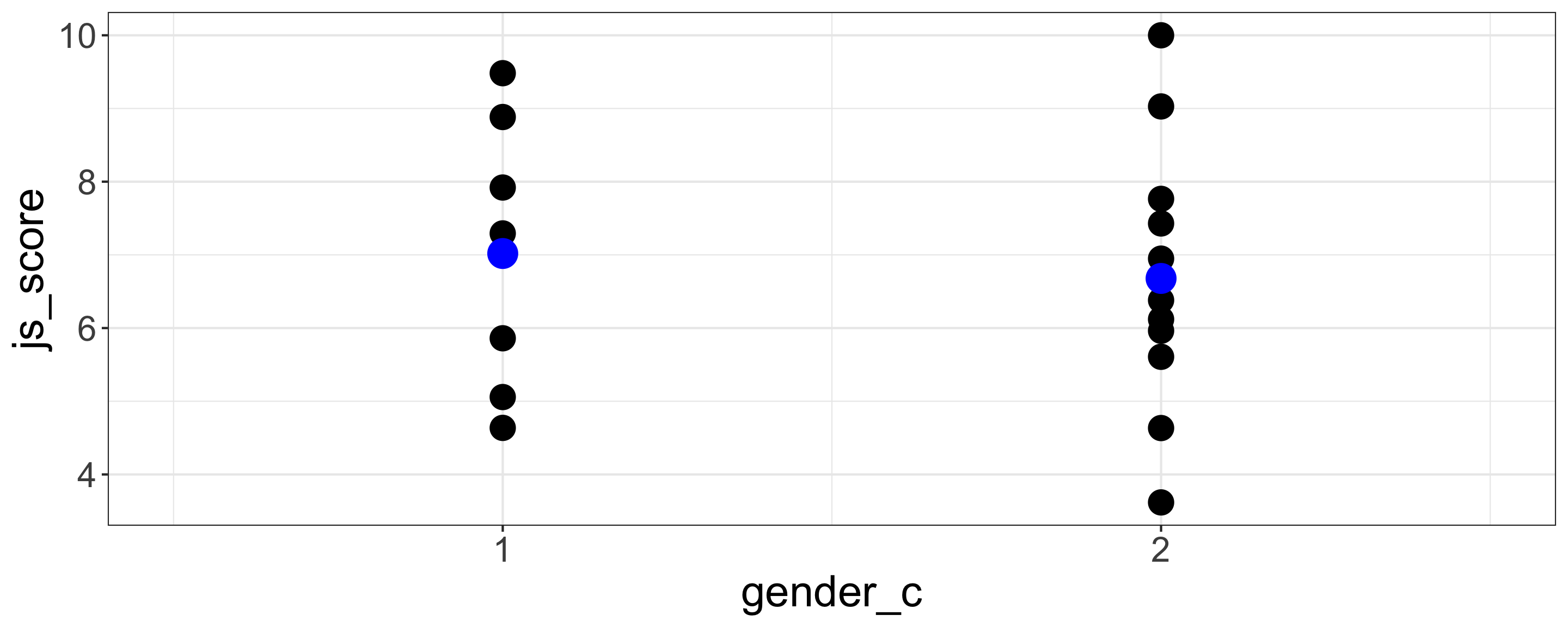
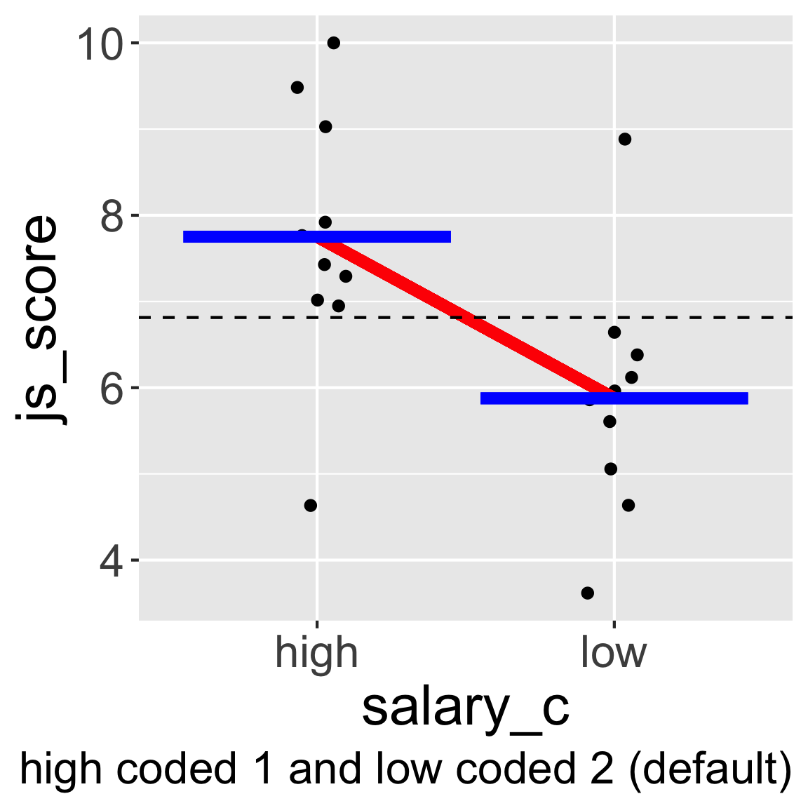
Comparing the difference between two averages is the same as comparing the slope of the line crossing these two averages:
- If two averages are not equal, then the slope of the line crossing these two averages is not 0
- If two averages are equal, then the slope of the line crossing these two averages is 0
Categorical Predictor with 2 Categories
Warning
JAMOVI and other software automatically code categorical variable following alphabetical order but sometimes you need to change these codes.
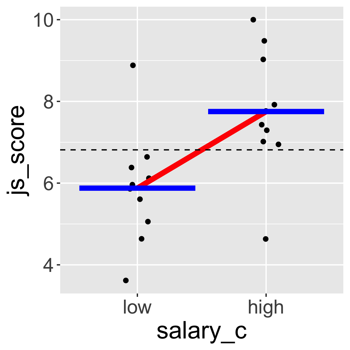
For example, here low coded with the value 1 and high coded with the value 2 would make more sense.
The way how categorical variables are coded will influence the sign of the estimate (positive vs. negative)
But it doesn’t change the value of the statistical test nor the \(p\)-value obtained
Testing Categorical Predictors
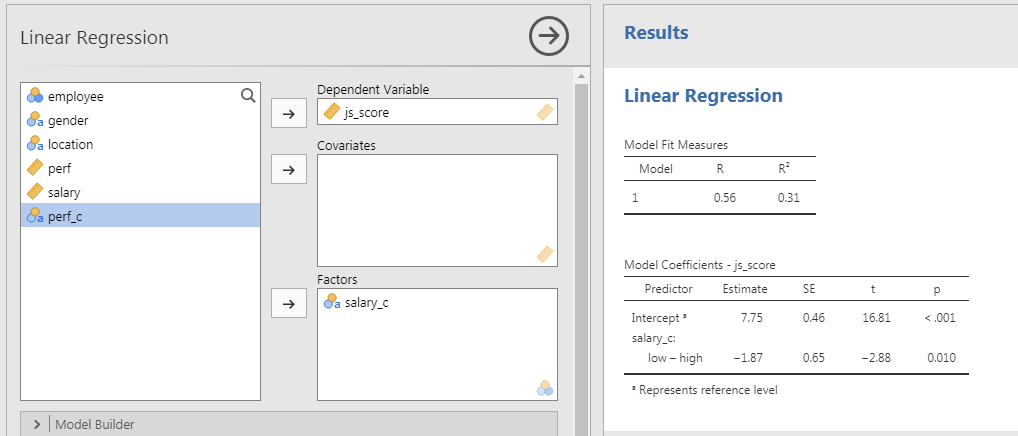
In JAMOVI
- Open your file
- Set variables in their correct type
- Analyses > Regression > Linear Regression
- Set \(js\_score\) as DV and \(salary\_c\) as Factors (i.e., Cat. Predictor)
Dummy Coding in Linear Regression
Dummy Coding is when a category is coded 0 and the other coded 1.
For example, in JAMOVI recode female as 0 and male as 1 (Dummy Coding): IF(gender == "female", 0, 1)
Dummy Coding is useful because one of the category becomes the intercept and is tested against 0.
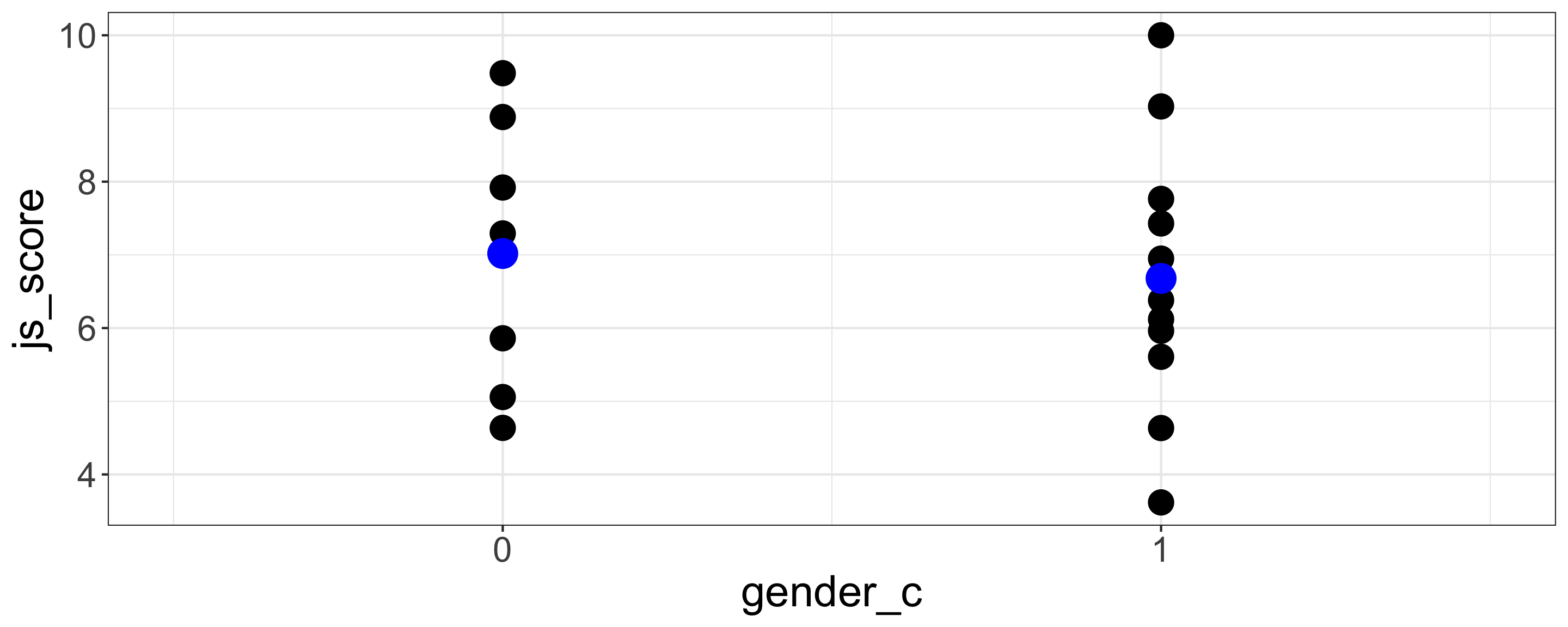
| term | estimate | std.error | statistic | p.value |
|---|---|---|---|---|
| (Intercept) | 7.02 | 0.62 | 11.33 | <0.001 |
| gender_c | -0.34 | 0.80 | -0.43 | 0.675 |
Deviation Coding in Linear Regression
Female = -1 and Male = 1
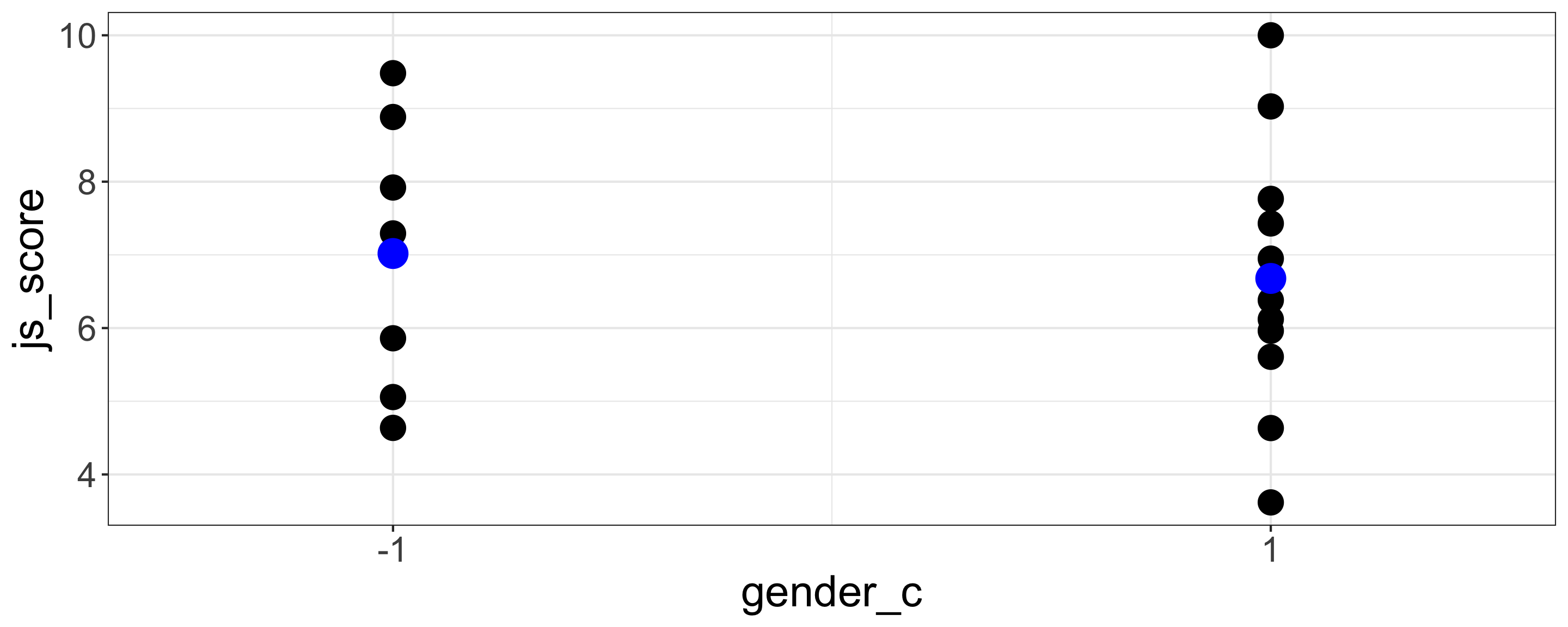
| term | estimate | std.error | statistic | p.value |
|---|---|---|---|---|
| (Intercept) | 6.85 | 0.4 | 17.12 | <0.001 |
| gender_c | -0.17 | 0.4 | -0.43 | 0.675 |
Female = -0.5 and Male = 0.5
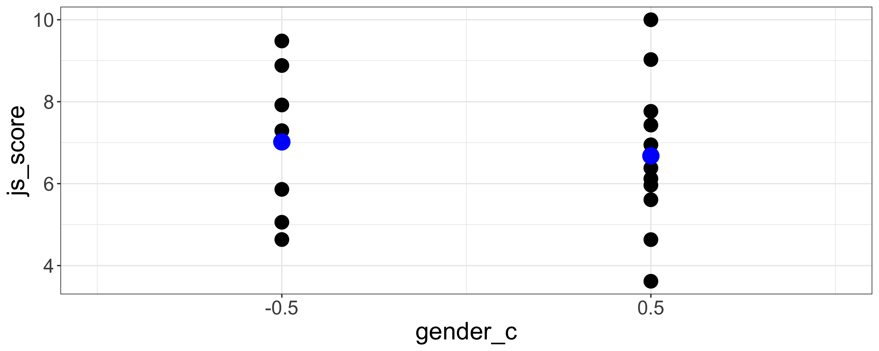
| term | estimate | std.error | statistic | p.value |
|---|---|---|---|---|
| (Intercept) | 6.85 | 0.4 | 17.12 | <0.001 |
| gender_c | -0.34 | 0.8 | -0.43 | 0.675 |
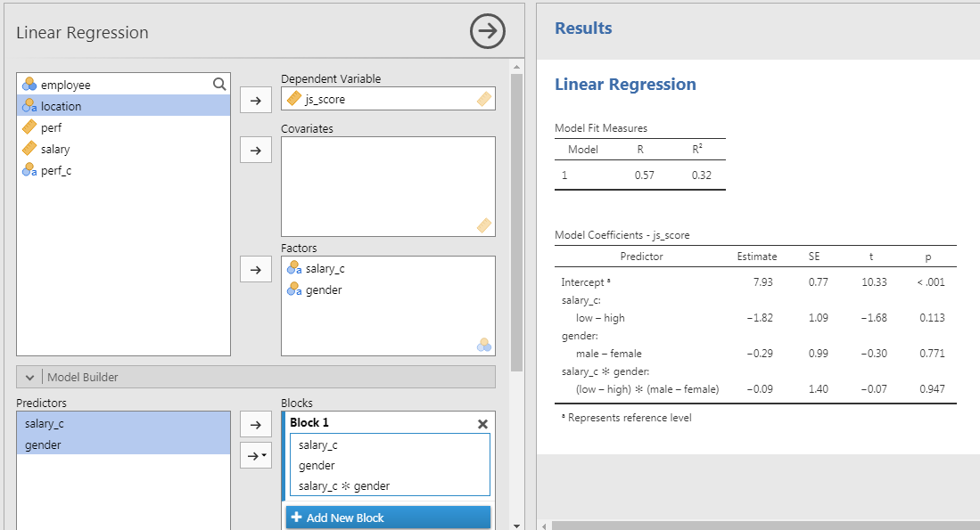
Interaction with Categorical Predictors
Categorical Predictor with 3+ Categories
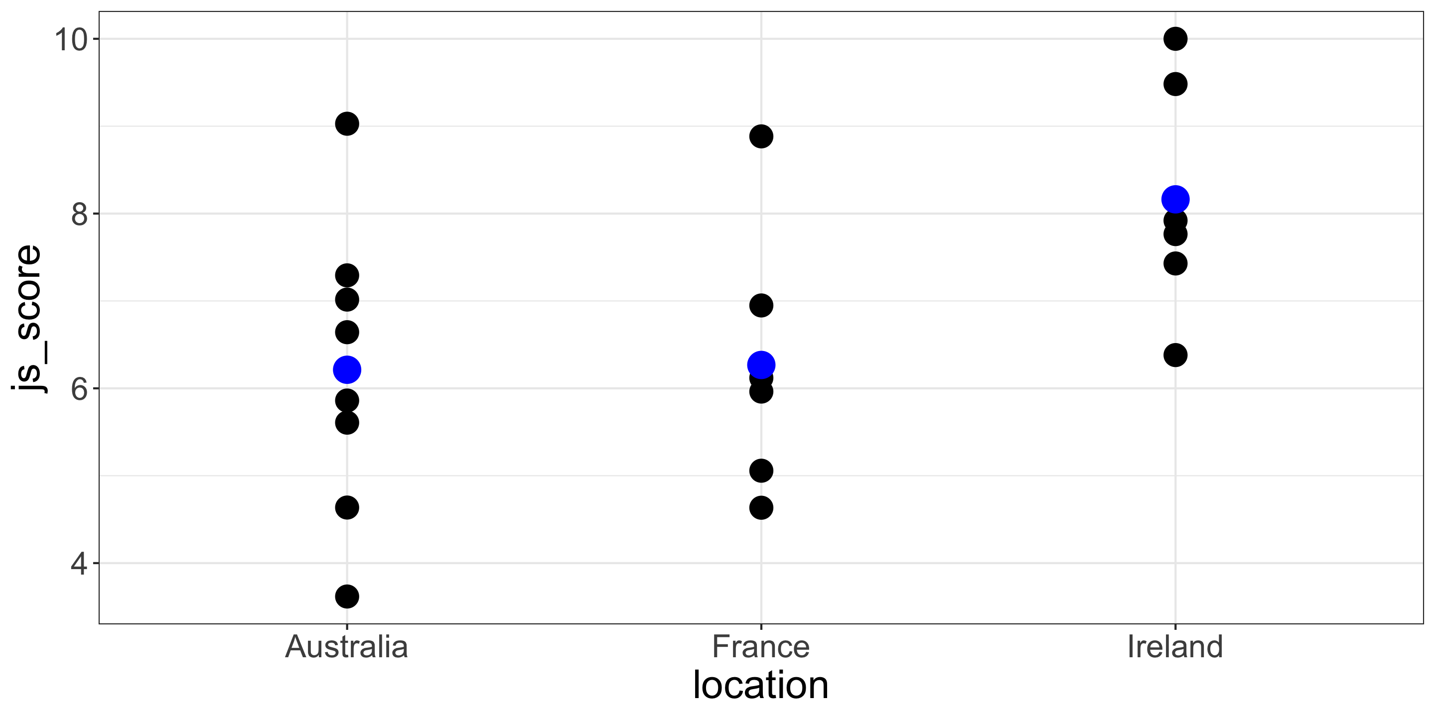
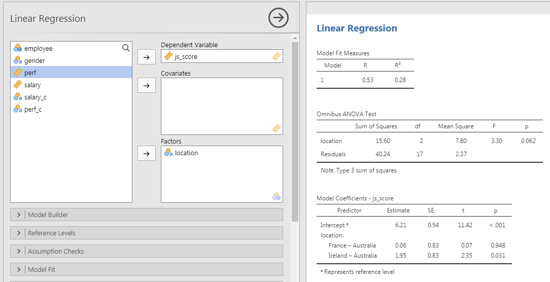
I would like to test the effect of the variable \(location\) which has 3 categories: “Ireland”, “France” and “Australia”.
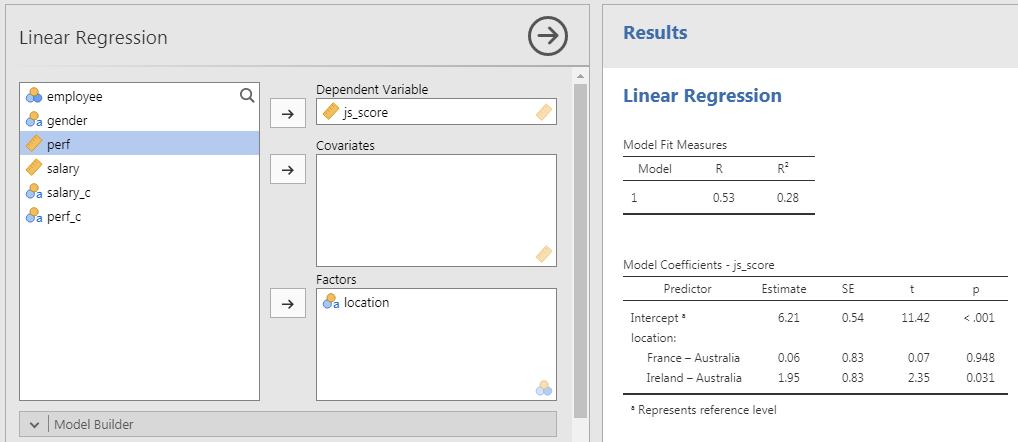
In the Model Coefficient Table, to test the estimate of \(location\), there is not 1 result for \(location\) but 2!
- Comparison of “Australia” vs. “France”
- Comparison of “Australia” vs. “Ireland”
Why multiple \(p\)-value are provided for the same predictor?
Coding Predictors with 3+ categories
Variables
- Outcome = \(js\_score\) (from 0 to 10)
- Predictor = \(location\) (3 categories: Australia, France and Ireland)
| employee | location | js_score |
|---|---|---|
| 1 | France | 5.057311 |
| 2 | Australia | 6.642440 |
| 3 | France | 6.119694 |
| 4 | Ireland | 9.482198 |
| 5 | France | 8.883347 |
| 6 | Australia | 7.015606 |
| 7 | France | 4.633738 |
| 8 | Ireland | 7.919998 |
| 9 | Australia | 9.028004 |
| 10 | Australia | 5.860449 |
| 11 | Ireland | 10.000000 |
| 12 | Australia | 3.617721 |
| 13 | France | 6.948510 |
| 14 | Ireland | 7.429012 |
| 15 | Australia | 7.292992 |
| 16 | Ireland | 7.765043 |
| 17 | Ireland | 6.380634 |
| 18 | France | 5.962925 |
| 19 | Australia | 5.607226 |
| 20 | Australia | 4.635931 |
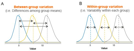
ANOVA Test for Overall Effects
I won’t go too much in the details but to check if at least one group is different from the others, the distance of each value to the overall mean (Between−group variation) is compared to the distance of each value to their group mean (Within−group variation).
If the Between−group variation is the same as the Within−group variation, all the groups are the same.
ANOVA in our Example
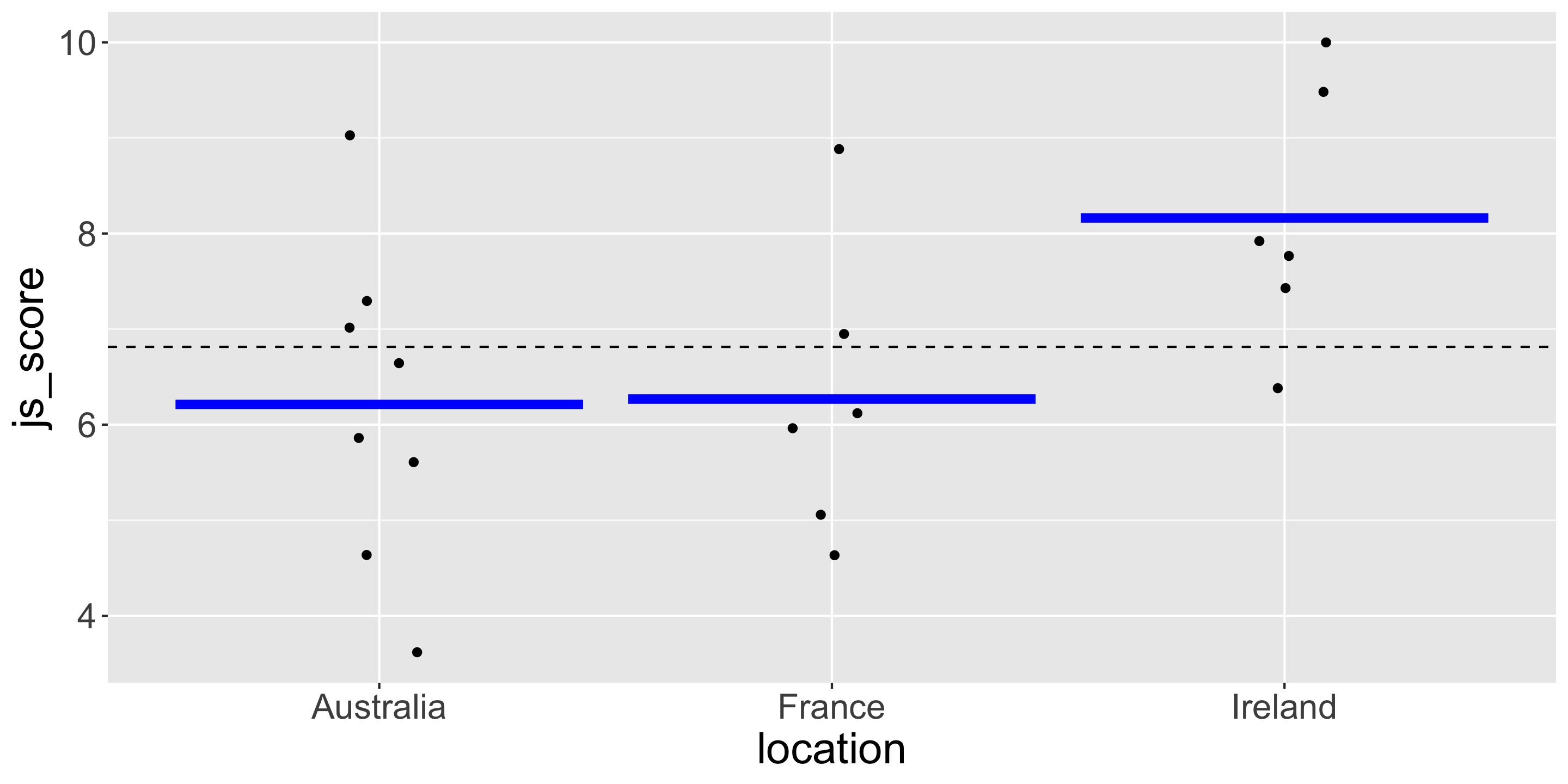
ANOVA in our Example
Results
There is no significant effect of employee’s \(location\) on their average \(js\_score\) ( \(F(2, 17) = 3.30\), \(p = .062\))
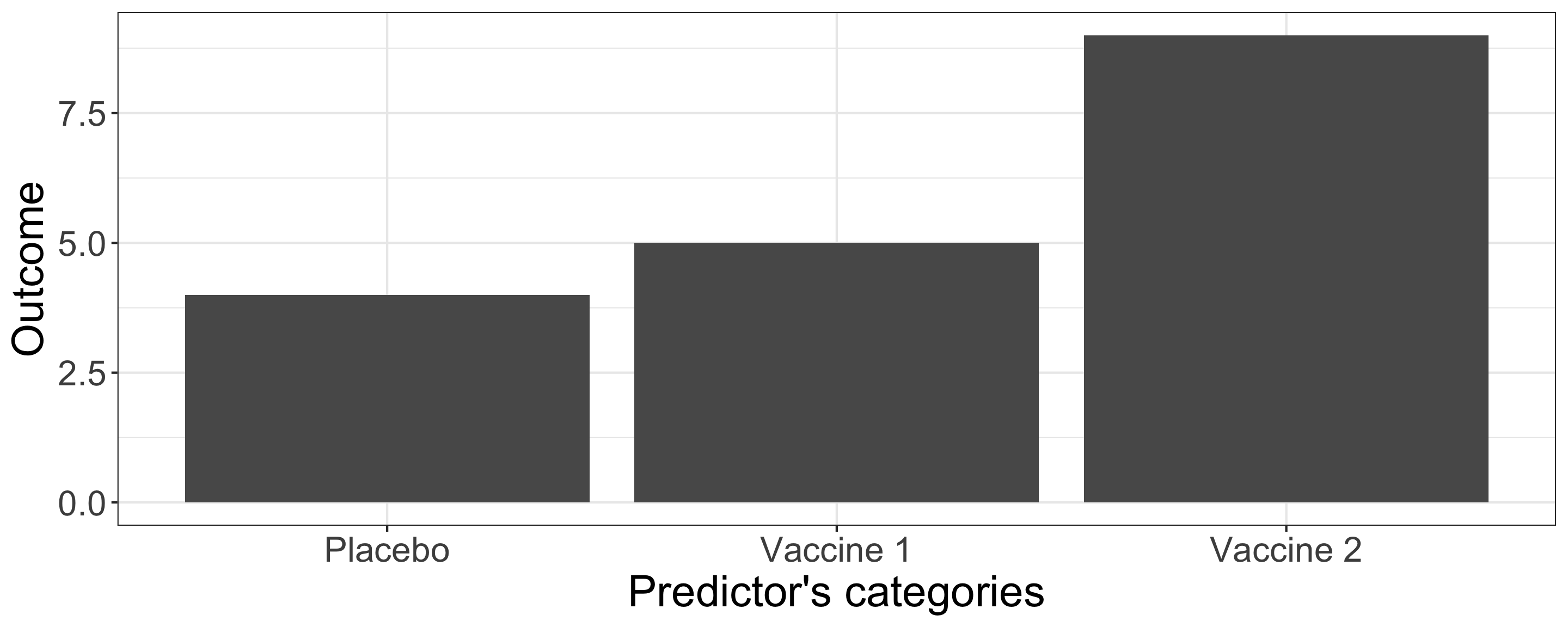
Sum to Zero Contrasts
Also called “Simple” contrast, each contrast encodes the difference between one of the groups and a baseline category, which in this case corresponds to the first group:
| Predictor's categories | Contrast1 | Contrast2 |
|---|---|---|
| Placebo | -1 | -1 |
| Vaccine 1 | 1 | 0 |
| Vaccine 2 | 0 | 1 |
Polynomial Contrasts
They are the most powerful of all the contrasts to test linear and non linear effects: Contrast 1 is called Linear, Contrast 2 is Quadratic, Contrast 3 is Cubic, Contrast 4 is Quartic …
| Predictor's categories | Contrast_1 | Contrast_2 |
|---|---|---|
| Low | -1 | 1 |
| Medium | 0 | -2 |
| High | 1 | 1 |

Thanks for your attention
and don’t hesitate to ask if you have any questions!