STA1005 - Quantitative Research Methods

Lecture 2: Understanding Models and Equations

Damien Dupré | DCU Business School

Essential Concepts to Master

In research outputs, all sections are linked:

flowchart LR
  A[Introduction] --> B[Literature<br>Review]
  B --> C[Methods]
  C --> D[Results]
  D --> E[Discussion &<br>Conclusion]

To understand the statistics in the results section it is essential to identify the concepts presented in each section:

flowchart LR
  A[Introduction] -- Variables --> B[Literature<br>Review]
  B -- Hypotheses --> C[Methods]
  C -- Model &<br>Equation --> D[Results]
  D -- Statistical<br>Test--> E[Discussion &<br>Conclusion]

1. Model Representation in the Method Section of Academic Reseach Paper

Method Section in Academic Papers

The method section is always structured in the same way:

1. Observations

Short section presenting where the data are coming from. If they are coming from human participants, then their average age and gender is indicated.

2. Variables

Short section presenting each variable as well as their type and role.

3. Procedure

Short section presenting how data were collected.

4. Data Analytics

Short section to display how the hypotheses are tested by displaying a graphical representation of the Model and its corresponding Equation(s).

Model Representation

Models are an overview of the predicted relationship between variables stated in the hypotheses

You must follow these rules:

Rule 1: All the arrows correspond to an hypothesis to be tested
Rule 2: All the tested hypotheses have to be represented with an arrow
Rule 3: Hypotheses using the same Outcome variable should be included in the same model
Rule 4: Only one Outcome variable is included in each model (except for SEM model)

Model Representation

A simple arrow is a main effect

A crossing arrow is an interaction effect

Note: By default, an interaction effect involves the test of the main effect hypotheses of all Predictors involved

Structure of Models

Distinguish square and circles

squares are actual measures/items
circles are latent variables related to measures/items

Example:

$Salary$ is directly measured (in $, €, or £) so it’s a square.
$Job\,Satisfaction$ is a latent variable with several questions so it’s a circle.

Items used for latent variables can be omitted in a model, variables are the most important.

Main Effect Relationship

Relationship between one Predictor and one Outcome variable

This model tests one main effect hypothesis

Relationship between two Predictors and one Outcome variable

This model tests two main effect hypotheses

Interaction Effect Relationship

An interaction means that the effect of a Predictor 1 on the Outcome variable will be different according the possibilities of a Predictor 2 (also called Moderation).

Effects representation:

Exactly the same results:

This model tests three hypotheses: 2 main effects and 1 interaction effect

Types of Model

Simple Model

One or more predictors
Only one outcome
Made of main or/and interaction effects

Mediation Model (simple or moderated)

At least 2 predictors (one call Mediator)
Only one outcome
Made of main effects only for simple mediation / main and interaction effects for moderated mediation

Structural Equation Model (SEM)

At least 2 predictors (usually latent variables)
One or more outcome
Made of main or/and interaction effects

Simple Model

Simple Models are the most statistically powerful, easy to test and reliable models. Always prefer a simple model compared to a more complicated solution.

Warning

Including interaction effect requires a significantly higher sample size.

Example:

This model tests four hypotheses:

3 main effects
1 interaction effect

Mediation Models

A Mediation model is a complex path analysis between 3 variables, where one of them explains the relationship between the other two. It is usually used to identify cognitive process in psychology.

Example:

This model tests one hypothesis:

1 mediation effect
but it requires 2 main effects

Structural Equation Model

A Structural Equation Model (SEM) is a complex path analysis between multiple variables including multiple Outcomes and using factor analysis for latent variable estimation.

Item contribution to a latent variable

The relationship between items of a scale and their corresponding latent variable is considered as significant by default if the scale is valid

For example, this model tests four hypotheses

A Good Model

Comprehensiveness: Explains a wide range of phenomena
Internal Consistency: Propositions and assumptions are consistent and fit together in a coherent manner
Parsimony: Contains only those concepts and assumptions essential for the explanation of a phenomenon
Testability: Concepts and relational statements are precise.
Empirical Validity: Holds up when tested in the real world.

A Good Model

Example:

A Bad Theory/Model

Too complicated
Does not explain many things
Cannot be tested

Is it bad?

Representing a Model

The representation of a model can easily be done directly in a manuscript written with Microsoft Words

For more details, is it also possible to draw the model in Microsoft PowerPoint and to copy-paste it in Microsoft Words.

Warning

Do NOT fill boxes with any color, use only black and white colors.
Use line arrow, no thick arrows allowed.

Representing a Model

Beside MS Words and PowerPoint, there are some ways to draw models in a nicer way.

Flowchart Software/Websites

There are many of them and google would find them very quickly but to my knowledge, https://www.diagrams.net/ is free, easy to use and very efficient.

Representing a Model

Flowchart Coding Languages

Going further into details of how to design academic models, flowchart coding languages are the ultimate steps.

Instead of using a GUI, it is possible to draw models from a couple of lines of code which is faster after practising a lot.

To my knowledge, the main flowchart coding language tool implementing the DOT style are:

But many more alternative can be used

DOT Language

It is easy to start by following these rules:

Variable names must not include space between words
Arrows are represented by the characters - and >

What you type:

digraph {
  "Predictor 1" -> "Outcome"
  "Predictor 2" -> "Outcome"
}

What you get:

DOT Language

To modify the orientation and the shape of the box, add the following options:

digraph {
  graph [rankdir = LR]
  node [shape = box]
  
  "Predictor 1" -> "Outcome"
  "Predictor 2" -> "Outcome"
}

DOT Language

Unfortunately the way to plot an interaction is much trickier. You have to include an invisible box to design the arrow crossing the main arrow:

digraph {
  graph [rankdir = LR]  
  node [shape = box]
  "Predictor 1"; "Predictor 2"; "Outcome"
  node [shape = point, width = 0, height = 0]
  ""
  
  "Predictor 2" -> ""
  "Predictor 1" -> "" [arrowhead = none]
  "" -> Outcome
  
  subgraph {
    rank = same; "Predictor 2"; "";
  }
}

There are many more rules to make more complicated models, see for more details https://graphviz.org/doc/info/lang.html

DotUML Extension for Google Docs

This DOT language can easily be implemented with the DotUML extension in Google Docs.

DotUML is developed by a company called BML Solutions but as far as I know it is a free plug-in (at least free of money).

See https://dotuml.com for more details.

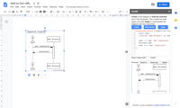
After installed the extension, use GraphViz and remove the code corresponding to the default example.

️ Your Turn!

In the research paper you have selected, draw the model(s) tested.

Remember, there is only 1 Outcome variable per model and it is not possible to draw two models with the same Outcome variable.

Send me your figure by email at damien.dupre@dcu.ie before the next lecture.

2. Understanding the Equation used to Test Hypotheses

A Basic Equation

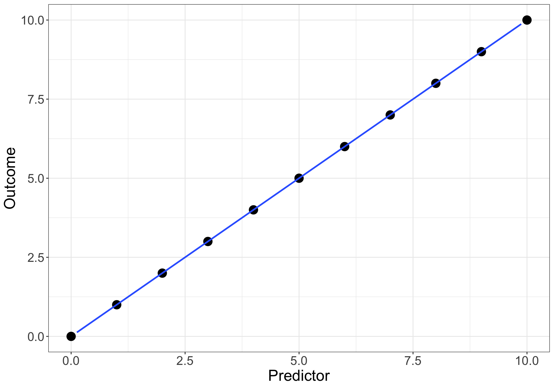
Let’s imagine the perfect scenario: your predictor Predictor variable explains perfectly the outcome variable.

The corresponding equation is: $Outcome = Predictor$

Observation	Outcome	Predictor
a	10	10
b	9	9
c	8	8
d	7	7
e	6	6
f	5	5
g	4	4
h	3	3
i	2	2
j	1	1
k	0	0

A Basic Equation

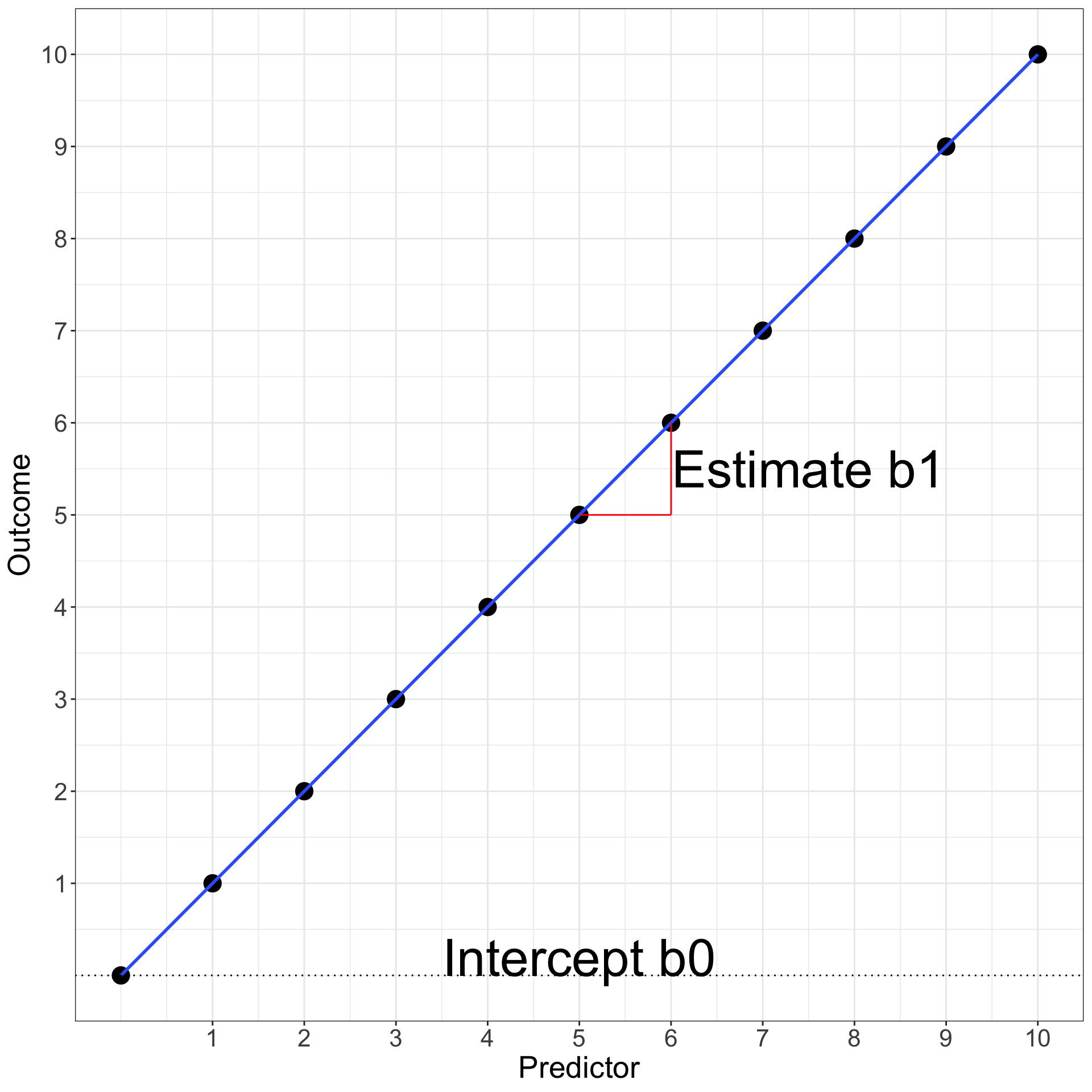
In the equation $Outcome = Predictor$, three coefficients are hidden because they are unused:

the intercept coefficient $b_{0}$ (i.e., the value of the Outcome when the Predictor = 0) which is 0 in our case
the estimate coefficient $b_{1}$ (i.e., how much the Outcome increases when the Predictor increases by 1) which is 1 in our case
the error coefficient $e$ (i.e., how far from the prediction line the values of the Outcome are) which is 0 in our case

A Basic Equation

So in general, the relation between a predictor and an outcome can be written as: \[Outcome = b_{0} + b_{1}\,Predictor + e\]

which is in our case:

\[Outcome = 0 + 1 * Predictor + 0\]

A Basic Equation

The equation $Outcome = b_{0} + b_{1}\,Predictor + e$ is the same as the good old $y = ax + b$ (here ordered as $y = b + ax$) where $b_{0}$ is $b$ and $b_{1}$ is $a$.

It is very important to know that under EVERY statistical test, a similar equation is used (t-test, ANOVA, Chi-square are all linear regressions).

Relationship between Variables

Relationship between a $Predictor$ and an $Outcome$ variable (stated in a main effect hypothesis or in an interaction effect hypothesis) is analysed in terms of:

“How many units of the Outcome variable increases/decreases/changes when the Predictor increases by 1 unit?”

For example:

How much Job Satisfaction increases when the Salary increases by €1?

Relationship between Variables

The value of how much of the Outcome variable changes:

Is called the Estimate (also called Unstandardised Estimate)
Uses the letter $b$ in equations (e.g., $b_1$, $b_2$, $b_3$, …)

For example:

If Job Satisfaction increases by 0.1 on a scale from 0 to 5 when the Salary increases by €1, then b associated to Salary is 0.1

Significance of Relationships

To evaluate if the strength of the relationship $b$ between a Predictor and an Outcome variable is significant, an equation is statistically tested using all the predictors related to the same Outcome.

The basic equation of a statistical model is:

\[Outcome = b_0 + b_n \,Predictors + Error\]

where the $Predictors$ includes all the $n$ variables used as predictor in formulated hypotheses using this specific $Outcome$ variable and being associated to a specific $b$ estimate.

Significance of Relationships

\[Outcome = b_0 + b_n \,Predictors + Error\]

This expresses the idea that:

The Outcome can be described by one or multiple predictors.
The remaining part of the Outcome’s variability that is not explained by the predictors is call the Error.

Equations, Variables and Effect Types

Except in special cases:

An Outcome (or Dependent Variable) has to be Continuous
A Predictor can be Continuous or Categorical

Example:

\[Job\,Satisfaction = b_{0} + b_{1}\,Salary + b_{2}\,Origin + e\]

In this equation, $Salary$ is continuous with a main effect on $Job\,Satisfaction$ ($b_{1}$) and $Origin$ is categorical with a main effect on $Job\,Satisfaction$ ($b_{2}$)

Equations, Variables and Effect Types

An interaction effect is represented by multiplying the 2 predictors involved:

\[Job\,Satisfaction = b_{0} + b_{1}\,Salary + b_{2}\,Origin + b_{3}\,Salary*Origin + e\]

In this equation, $Salary$ is continuous with a main effect on $Job\,Satisfaction$ ($b_{1}$), $Origin$ is categorical with a main effect on $Job\,Satisfaction$ ($b_{2}$), and $Salary$ with $Origin$ have an interaction effect on $Job\,Satisfaction$ ($b_{3}$)

Relevance of the Intercept

To test hypotheses, only the $b$ values associated to Predictors / Independent Variables are important.

The intercept is always included in an equation but its result is useless for hypothesis testing.

Let’s see why the intercept is always included but discarded most of the time.

Relevance of the Intercept

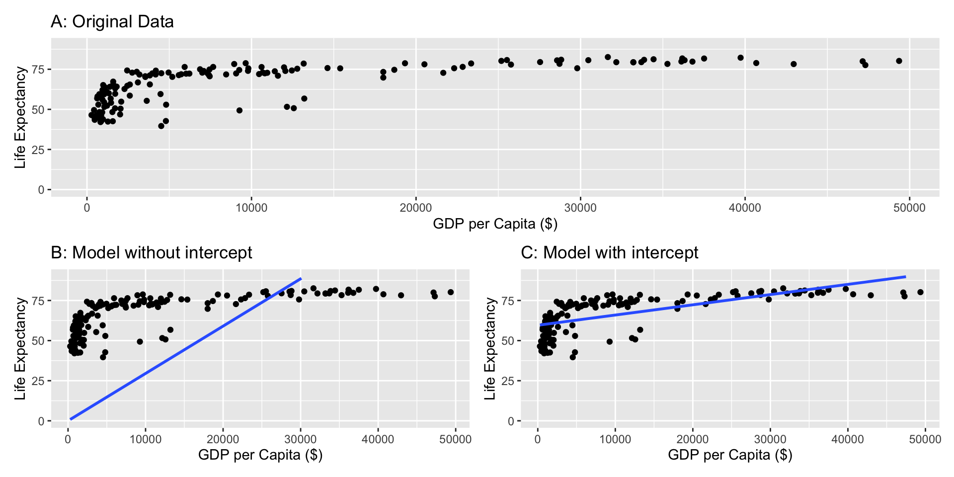
Imagine we want to test the relationship between GDP per Capita and Life Expectancy of countries in the world. Let’s compare a model without and a model with intercept:

Without intercept: $Life\,Expectancy = b_{1}\,GDP\,per\,Capita + e$
With intercept: $Life\,Expectancy = b_{0} + b_{1}\,GDP\,per\,Capita + e$

Relevance of the Intercept

If the intercept is not included, the intercept is zero and can lead to estimation errors

Notes on the Equations

1. Greek or Latin alphabet?

\[Y = \beta_{0} + \beta_{1}\,X_{1} + \epsilon \; vs. \; Y = b_{0} + b_{1}\,X_{1} + e\]

2. Subscript $i$ or not?

\[Y = b_{0} + b_{1}\,X_{1} + e \; vs. \; Y_{i} = b_{0} + b_{1}\,X_{1_{i}} + e_{i}\]

3. Which sign between estimates and predictors?

\[Y = b_{0} + b_{1}.X_{1} + b_{2}*X_{2} + b_{3}\,X_{3} + e\]

4. Hat on $Y$ or not? Capital letter or not?

\[\hat{Y}\; or\; \hat{y}\; vs.\; Y\; or\; y\]

Representing an Equation

Exactly like with models, there are different ways to communicate an equation in Academic research outputs.

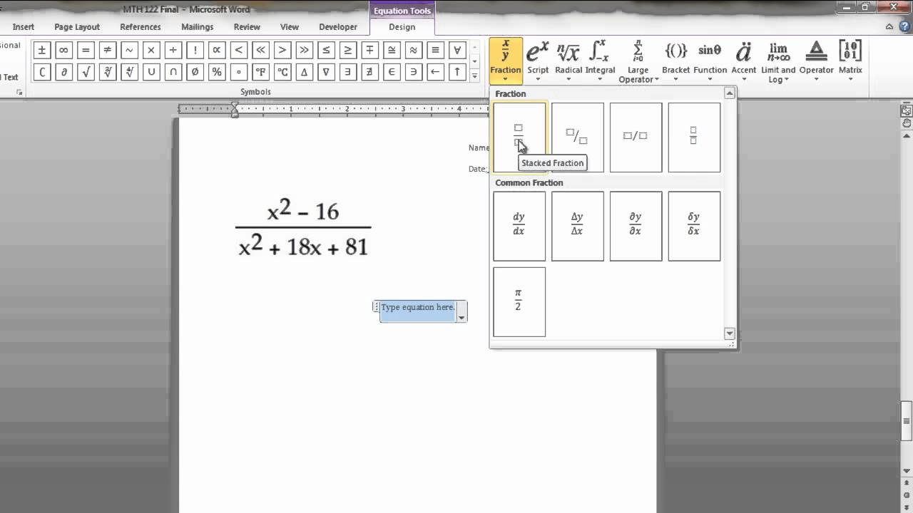
The least sophisticated approach would be to type the equation in Microsoft Words and to apply some italics and subscript style a posteriori.

While there is nothing wrong with this approach, note that Microsoft Words has a tool to insert equations (Insert -> Equations), then a GUI will help you to design special characters in equations.

Representing an Equation

Now there is a better way, which is also more complicated.

$\LaTeX$ is used for entire manuscripts with all the specific design requirements imposed by ths style of academic journals. LaTex is the hell and we will see a specific approach to avoid it but the LaTex style for equations is the best.

Representing an Equation

Here are the most basic rules:

Starts with \begin{equation} and ends with \end{equation}
Space between words can be added with \,
To subscript a number use the underscore sign _

For example:

\begin{equation}
  Outcome = b_0 + b_1\,Predictor 1 + b_2\,Predictor 2 + e
\end{equation}

Is translated as:

\[Outcome = b_0 + b_1\,Predictor 1 + b_2\,Predictor 2 +e\]

Auto-LaTeX Equations for Google Docs

Another fantastic extension is available for Google Docs called Auto-LaTeX Equations

Instead of using \begin{equation} and \end{equation}, use $$ to open and close the equation

Then, click on “Render Equation”, for the equation to be transformed in LaTex style

Note that some website can help to create the latex code, see for example https://latex.codecogs.com/eqneditor/editor.php

️ Your Turn!

I will show you some results. Using these results:

Identify the role of variables,
Formulate the tested hypotheses
Draw the corresponding model, and
Translate it in an equation

Example 1

Using the results obtained, identify the role of variables, formulate the tested hypotheses, draw the corresponding model, and translate it in an equation

Data

Participant	Sleep Time	Exam Results
ppt1	9.0	89
ppt2	5.0	64
ppt3	8.5	71
ppt4	7.0	77
ppt5	6.5	78
ppt6	5.5	69

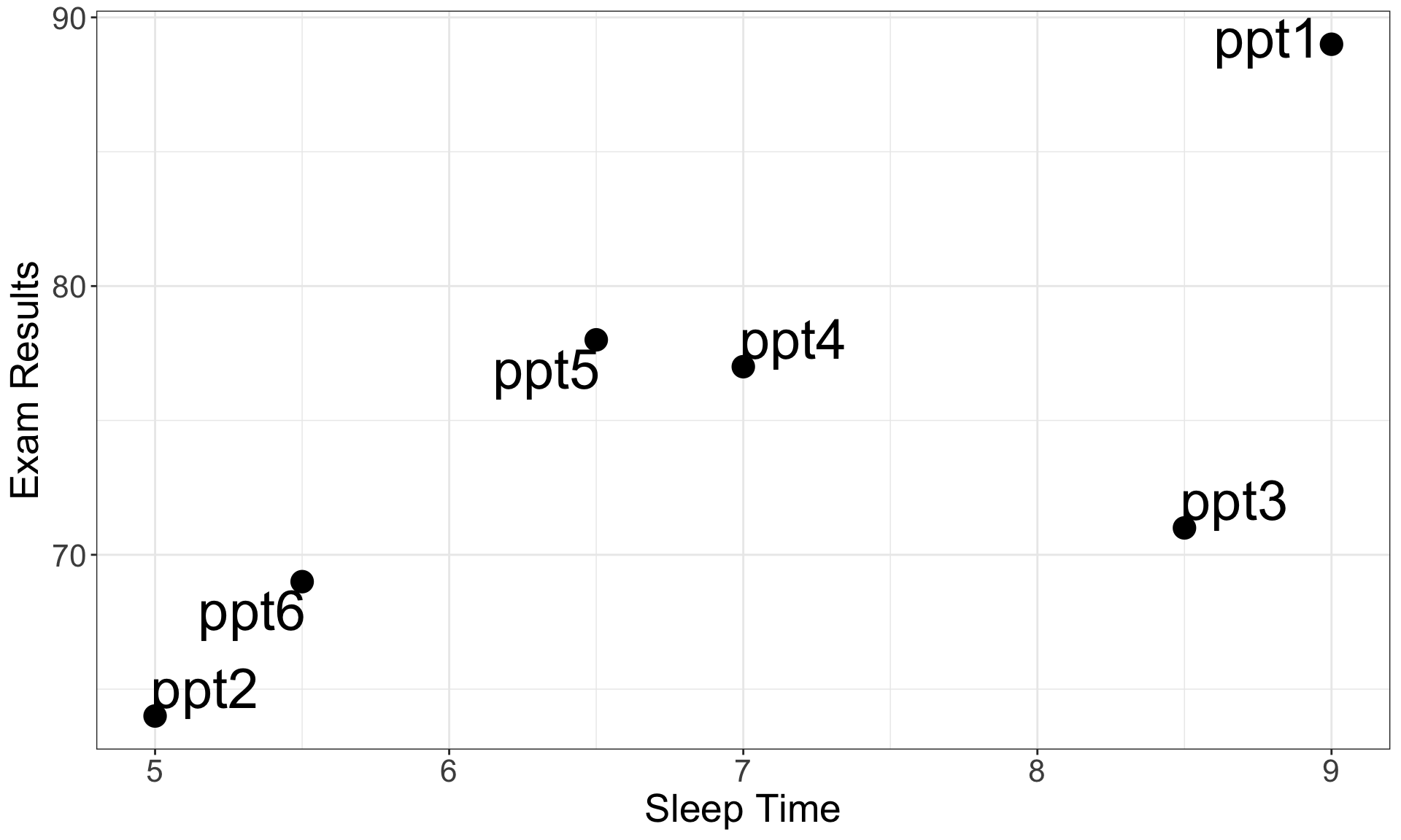
Visualisation

05:00

Example 1

Variables:

Outcome = Exam Results (from 0 to 100)
Predictor = Sleep Time (from 0 to Inf.)

Alternative Hypothesis:

$H_a$: Exam Results increases when Sleep Time increases
($H_0$: Exam Results stay the same when Sleep Time increases)

Example 1

Model:

Equation:

\[Exam\,Results = b_{0} + b_{1}\,Sleep\,Time + e\]

Example 2

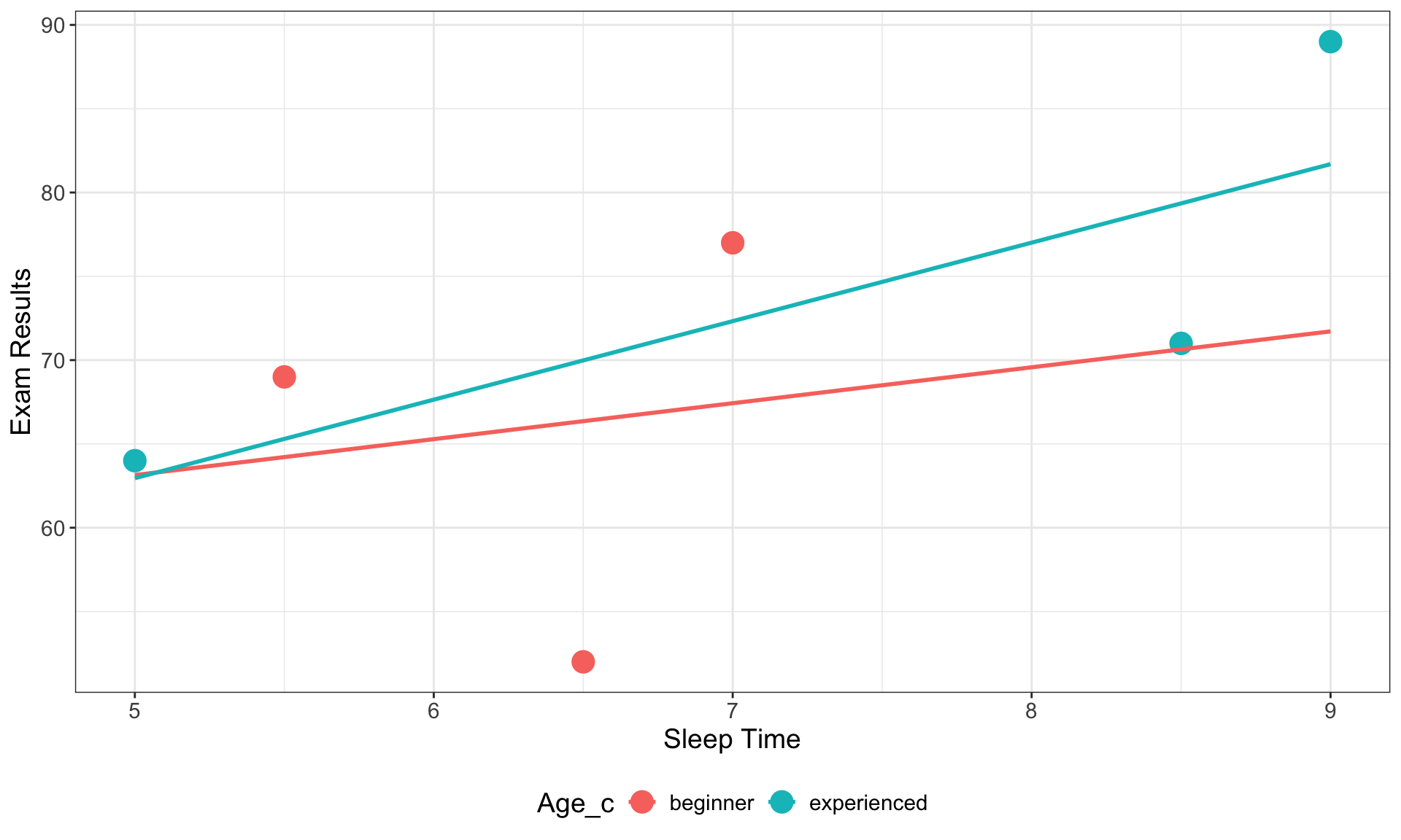
Using the results obtained, identify the role of variables, formulate the tested hypotheses, draw the corresponding model, and translate it in an equation

Data

Participant	Sleep Time	Exam Results	Age_c
ppt1	9.0	89	experienced
ppt2	5.0	64	experienced
ppt3	8.5	71	experienced
ppt4	7.0	77	beginner
ppt5	6.5	52	beginner
ppt6	5.5	69	beginner

Visualisation

05:00

Example 2

Variables:

Outcome = Exam Results (from 0 to 100)
Predictor 1 = Sleep Time (from 0 to Inf.)
Predictor 2 = Age (experienced vs beginner)

Alternative Hypotheses:

$H_{a_{1}}$: Exam Results increases when Sleep Time increases
$H_{a_{2}}$: Exam Results of experienced students are higher than for beginner students
$H_{a_{3}}$: The effect of Sleep Time on Exam Results is higher for experienced than for beginner students

Example 2

Model:

Classic Representation

Effects Correspondence

Equation:

\[Exam\,Results = b_{0} + b_{1}\,Sleep\,Time + b_{2}\,Age + b_{3}\,Sleep\,Time*Age + e\]

️ Your Turn!

In the research paper you have selected, write the equation(s) corresponding to the model(s)

Send me your equation(s) by email at damien.dupre@dcu.ie before the next lecture

Conclusion

Follow the Steps

Variables

Identify the role and type of each of your variables

Hypotheses

Formulate your alternative hypotheses by using the proposed templates
Any other formulation, even if it make sense, is not good practice (e.g. using the terms “has an impact”, “is related to”, “influences”, …)
An interaction hypothesis requires the formulation of the main effect hypothesis of each predictor involved

Model

A model should represent all your hypotheses and only your hypotheses
Draw only model per Outcome variable (except is doing SEM analyses)
Use the same names or acronyms as your hypotheses

Equation

Formulate your equation(s) in every paper that you want to submit (if reviewers want to remove it, they will tell you)

Thanks for your attention

and don’t hesitate to ask if you have any questions!

@damien-dupre
@damien-dupre

https://damien-dupre.github.io
damien.dupre@dcu.ie

STA1005 - Quantitative Research Methods

Essential Concepts to Master

1. Model Representation in the Method Section of Academic Reseach Paper

Method Section in Academic Papers

1. Observations

2. Variables

3. Procedure

4. Data Analytics

Model Representation

Model Representation

Structure of Models

Main Effect Relationship

Interaction Effect Relationship

Types of Model

Simple Model

Mediation Model (simple or moderated)

Structural Equation Model (SEM)

Simple Model

Mediation Models

Structural Equation Model

A Good Model

A Good Model

A Bad Theory/Model

Representing a Model

Representing a Model

Representing a Model

DOT Language

DOT Language

DOT Language

DotUML Extension for Google Docs

️ Your Turn!

2. Understanding the Equation used to Test Hypotheses

A Basic Equation

A Basic Equation

A Basic Equation

A Basic Equation

Relationship between Variables

Relationship between Variables

Significance of Relationships

Significance of Relationships

Equations, Variables and Effect Types

Equations, Variables and Effect Types

Relevance of the Intercept

Relevance of the Intercept

Relevance of the Intercept

Notes on the Equations

1. Greek or Latin alphabet?

2. Subscript \(i\) or not?

3. Which sign between estimates and predictors?

4. Hat on \(Y\) or not? Capital letter or not?

Representing an Equation

Representing an Equation

Representing an Equation

Auto-LaTeX Equations for Google Docs

️ Your Turn!

Example 1

Example 1

Example 1

Example 2

Example 2

Example 2

️ Your Turn!

Conclusion

Follow the Steps

Variables

Hypotheses

Model

Equation